AlexNetAlexNet
Krizhevsky, Sutskever, Hinton. ImageNet Classification with Deep Convolutional Neural Networks. NeurIPS 2012.
1. 왜 나왔나? (Problem)
2012년 이전의 이미지 분류는 사람이 특징을 설계하는 방식이었다. SIFT, HOG 같은 특징 추출기로 이미지를 벡터로 바꾸고, 그 위에 SVM 같은 분류기를 얹었다. 이 방식은 두 가지 벽에 부딪혀 있었다.
- 성능 정체: 특징을 사람이 만들다 보니 복잡한 이미지에서 한계가 뚜렷했다. ImageNet 대회 top-5 오류율은 25% 근처에서 맴돌았다.
- 신경망은 “이론상 좋지만 실제로는 안 되는” 기술: CNN은 LeNet(1998)부터 있었지만 손글씨 숫자 같은 작은 문제에서만 통했다. 네트워크를 깊고 크게 만들면
- 학습이 너무 느리고 (sigmoid/tanh의 기울기 포화, CPU 연산 한계)
- 데이터 대비 파라미터가 많아 과적합이 심했다.
즉 풀어야 할 문제는 이것이었다. “120만 장, 1000개 클래스짜리 대규모 데이터에서, 거대한 CNN을 현실적인 시간 안에, 과적합 없이 학습시킬 수 있는가?”
2. 다른 방법과 뭐가 다른가?
| 비교 대상 | 그쪽 방식 | AlexNet |
|---|---|---|
| 전통 방식 (SIFT + SVM) | 특징을 사람이 설계 | 특징을 데이터로부터 학습 (end-to-end) |
| LeNet-5 (1998) | 작은 입력(32×32), 층 얕음, 파라미터 약 6만, CPU, tanh | 224×224 컬러, Conv 5 + FC 3, 파라미터 약 6,000만, GPU, ReLU |
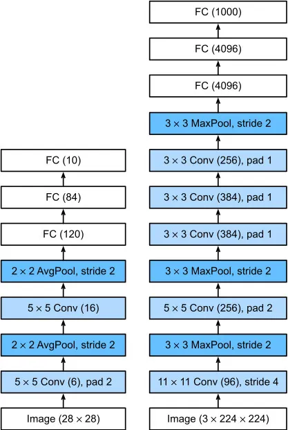
좌측은 LeNet-5, 우측은 AlexNet입니다. 이미지 출처: daeun-computer-uneasy.tistory.com
핵심 차이는 “새로운 층을 발명했다”가 아니라, 규모를 키웠을 때 생기는 문제들을 실전적으로 해결해서 깊은 CNN이 실제로 동작함을 증명했다는 점이다.
3. 그래서 어떻게 풀었나? (Solve)
구조: Conv 5층 + FC 3층
| 층 | 구성 | 비고 |
|---|---|---|
| Conv1 | 96개, 11×11, stride 4 | ReLU → LRN → MaxPool |
| Conv2 | 256개, 5×5 | ReLU → LRN → MaxPool |
| Conv3 | 384개, 3×3 | ReLU |
| Conv4 | 384개, 3×3 | ReLU |
| Conv5 | 256개, 3×3 | ReLU → MaxPool |
| FC6 | 4096 | ReLU + Dropout |
| FC7 | 4096 | ReLU + Dropout |
| FC8 | 1000 | Softmax |
문제별 해결책
학습이 느리다 → ReLU + GPU
max(0, x)는 양수 구간에서 기울기가 1로 유지돼 포화가 없다. 논문 실험에서 tanh 대비 같은 오류율 도달이 약 6배 빨랐다.- GTX 580(3GB) 한 장에 모델이 안 들어가서 네트워크를 절반씩 두 GPU에 나눠 학습했다. 특정 층에서만 GPU끼리 통신한다. (구조도가 위아래 두 갈래인 이유)
과적합이 심하다 → Dropout + Data Augmentation
- Dropout (p=0.5): FC6, FC7에서 뉴런을 무작위로 끈다. 파라미터가 몰린 FC층의 과적합을 직접 겨냥했다.
- Data Augmentation: 256×256에서 무작위 224×224 크롭 + 좌우 반전, PCA 기반 색상 변형으로 데이터를 사실상 크게 늘렸다.
일반화 성능을 조금 더 → Overlapping Pooling, LRN
- 3×3 풀링을 stride 2로 겹쳐서 적용.
- LRN으로 인접 채널 간 정규화. (단, 이후 효과가 미미하다고 밝혀져 BatchNorm에 자리를 내줌)
LRN(Local Response Normalization)이란? LRN은 AlexNet에서 사용한 정규화 기법이다. 같은 공간 위치에 있는 인접 채널들의 활성값을 이용해 각 값을 조정한다. 주변 채널의 활성값이 클수록 더 큰 값으로 나누기 때문에, 해당 채널의 출력이 작아진다. 여기서 값을 **‘누른다’**는 것은 0으로 만든다는 뜻이 아니라 크기를 줄인다는 뜻이다. 큰 활성값도 LRN을 거치면 작아질 수 있으며, 채널 사이의 반응을 상대적으로 비교하는 효과가 있다. AlexNet에서는 일부 합성곱 층의 ReLU 뒤, Max Pooling 앞에 LRN을 적용했다. 오늘날에는 LRN보다 Batch Normalization 같은 정규화 방법이 주로 사용된다.
Overlapping Pooling이란?
풀링 창을 이동할 때 인접한 창이 서로 겹치도록 하는 방식이다. 풀링 창의 크기보다 이동 간격(stride)이 작으면 겹침이 생긴다.
예를 들어 AlexNet은 3×3 Max Pooling에 stride 2를 사용했다. 첫 번째 창이 가로 방향의 13번째 값을 보면, 다음 창은 35번째 값을 본다. 3번째 값이 두 창에 모두 포함되는 것이다.
반대로 2×2 창을 stride 2로 이동하면 창끼리 겹치지 않는다. AlexNet 논문에서는 overlapping pooling을 사용했을 때 오류율이 소폭 낮아졌다고 보고했다.
학습 설정: SGD + momentum 0.9, weight decay 0.0005, batch 128, lr 0.01에서 시작해 정체 시 1/10, 약 90 epoch, 5~6일.
결과
ILSVRC 2012 top-5 오류율 15.3%. 2위는 26.2%. 이 격차로 컴퓨터 비전의 주류가 하루아침에 딥러닝으로 넘어갔다.
4. 코드로는 어떻게 쓰나?
실무에서 AlexNet을 처음부터 학습시킬 일은 거의 없다. 주로 구조를 직접 구현하며 CNN을 이해하는 용도나, 사전학습 모델로 전이학습을 연습하는 용도로 쓴다.
참고:
torchvision의 AlexNet은 원 논문이 아니라 단일 GPU 버전이다. Conv1 채널이 64개이고, LRN이 없다.
(1) 직접 구현 (PyTorch)
import torch
import torch.nn as nn

class AlexNet(nn.Module):
    def __init__(self, num_classes=1000):
        super().__init__()
        self.features = nn.Sequential(
            nn.Conv2d(3, 96, kernel_size=11, stride=4, padding=2),
            nn.ReLU(inplace=True),
            nn.LocalResponseNorm(size=5),
            nn.MaxPool2d(kernel_size=3, stride=2),     # overlapping pooling

            nn.Conv2d(96, 256, kernel_size=5, padding=2),
            nn.ReLU(inplace=True),
            nn.LocalResponseNorm(size=5),
            nn.MaxPool2d(kernel_size=3, stride=2),

            nn.Conv2d(256, 384, kernel_size=3, padding=1),
            nn.ReLU(inplace=True),
            nn.Conv2d(384, 384, kernel_size=3, padding=1),
            nn.ReLU(inplace=True),
            nn.Conv2d(384, 256, kernel_size=3, padding=1),
            nn.ReLU(inplace=True),
            nn.MaxPool2d(kernel_size=3, stride=2),
        )
        self.classifier = nn.Sequential(
            nn.Dropout(0.5),
            nn.Linear(256 * 6 * 6, 4096),
            nn.ReLU(inplace=True),
            nn.Dropout(0.5),
            nn.Linear(4096, 4096),
            nn.ReLU(inplace=True),
            nn.Linear(4096, num_classes),
        )

    def forward(self, x):
        x = self.features(x)
        x = torch.flatten(x, 1)
        return self.classifier(x)

model = AlexNet()
print(model(torch.randn(1, 3, 224, 224)).shape)  # torch.Size([1, 1000])
(2) 사전학습 모델로 추론
from torchvision.models import alexnet, AlexNet_Weights
from PIL import Image

weights = AlexNet_Weights.IMAGENET1K_V1
model = alexnet(weights=weights).eval()
preprocess = weights.transforms()   # 리사이즈·크롭·정규화를 한 번에

img = preprocess(Image.open("dog.jpg")).unsqueeze(0)
with torch.no_grad():
    pred = model(img).softmax(dim=1)

idx = pred.argmax().item()
print(weights.meta["categories"][idx], pred[0, idx].item())
(3) 전이학습: 내 데이터(예: 5개 클래스)에 맞추기
model = alexnet(weights=AlexNet_Weights.IMAGENET1K_V1)

# 특징 추출부는 고정
for p in model.features.parameters():
    p.requires_grad = False

# 마지막 FC층만 내 클래스 수로 교체
model.classifier[6] = nn.Linear(4096, 5)

optimizer = torch.optim.SGD(
    filter(lambda p: p.requires_grad, model.parameters()),
    lr=1e-3, momentum=0.9, weight_decay=5e-4,   # 논문 설정과 같은 계열
)
Krizhevsky, Sutskever, Hinton. ImageNet Classification with Deep Convolutional Neural Networks. NeurIPS 2012.
1. Why did it appear? (Problem)
Before 2012, image classification relied on features designed by people. Feature extractors like SIFT and HOG turned images into vectors, and a classifier such as an SVM sat on top. This approach had hit two walls.
- Stalled performance: because people hand-crafted the features, the limits were obvious on complex images. Top-5 error on the ImageNet challenge hovered around 25%.
- Neural networks were “good in theory, broken in practice”: CNNs had existed since LeNet (1998), but only worked on small problems like handwritten digits. Making the network deeper and larger meant
- training was far too slow (saturating sigmoid/tanh gradients, limited CPU compute), and
- there were so many parameters relative to the data that overfitting was severe.
So the problem to solve was this: “Can we train a huge CNN on a large dataset of 1.2 million images and 1,000 classes, in a realistic amount of time, without overfitting?”
2. How is it different from other approaches?
| Compared with | Their approach | AlexNet |
|---|---|---|
| Traditional (SIFT + SVM) | Features designed by people | Features learned from data (end-to-end) |
| LeNet-5 (1998) | Small input (32×32), shallow, ~60K parameters, CPU, tanh | 224×224 color, 5 Conv + 3 FC, ~60M parameters, GPU, ReLU |
LeNet-5 on the left, AlexNet on the right. Image source: daeun-computer-uneasy.tistory.com
The key difference is not that it “invented a new layer”, but that it solved, in practice, the problems that appear when you scale up, and proved that a deep CNN actually works.
3. So how did it solve it? (Solve)
Architecture: 5 Conv layers + 3 FC layers
| Layer | Configuration | Notes |
|---|---|---|
| Conv1 | 96 filters, 11×11, stride 4 | ReLU → LRN → MaxPool |
| Conv2 | 256 filters, 5×5 | ReLU → LRN → MaxPool |
| Conv3 | 384 filters, 3×3 | ReLU |
| Conv4 | 384 filters, 3×3 | ReLU |
| Conv5 | 256 filters, 3×3 | ReLU → MaxPool |
| FC6 | 4096 | ReLU + Dropout |
| FC7 | 4096 | ReLU + Dropout |
| FC8 | 1000 | Softmax |
A fix for each problem
Training is slow → ReLU + GPU
max(0, x)keeps a gradient of 1 in the positive range, so it does not saturate. In the paper’s experiment it reached the same error rate about 6× faster than tanh.- The model did not fit on a single GTX 580 (3GB), so they split the network in half across two GPUs. The GPUs only communicate at certain layers. (That is why the architecture diagram has two branches, top and bottom.)
Overfitting is severe → Dropout + Data Augmentation
- Dropout (p=0.5): randomly switches off neurons in FC6 and FC7, directly targeting overfitting in the FC layers where the parameters are concentrated.
- Data Augmentation: random 224×224 crops from 256×256 images, horizontal flips and PCA-based color jitter effectively enlarged the dataset by a lot.
A bit more generalization → Overlapping Pooling, LRN
- 3×3 pooling applied with stride 2 so the windows overlap.
- LRN normalizes across neighboring channels. (It was later shown to have little effect and gave way to BatchNorm.)
What is LRN (Local Response Normalization)? LRN is the normalization technique used in AlexNet. It adjusts each value using the activations of neighboring channels at the same spatial position. The larger the activations of the surrounding channels, the larger the divisor, so that channel’s output becomes smaller. Here, “suppressing” a value does not mean setting it to zero; it means shrinking it. Even a large activation can become smaller after LRN, which has the effect of comparing responses across channels relative to each other. AlexNet applied LRN after the ReLU and before max pooling in some convolutional layers. Today, normalization methods such as Batch Normalization are used instead of LRN.
What is Overlapping Pooling? It moves the pooling window so that adjacent windows overlap. If the stride is smaller than the window size, overlap occurs. For example, AlexNet used 3×3 max pooling with stride 2. If the first window covers values 1–3 horizontally, the next covers values 3–5, so the 3rd value is included in both windows. In contrast, a 2×2 window moved with stride 2 never overlaps. The AlexNet paper reported a slightly lower error rate with overlapping pooling.
Training setup: SGD + momentum 0.9, weight decay 0.0005, batch 128, learning rate starting at 0.01 and divided by 10 when it plateaued, about 90 epochs, 5–6 days.
Results
ILSVRC 2012 top-5 error of 15.3%, against 26.2% for second place. With that gap, mainstream computer vision moved to deep learning almost overnight.
4. How do you use it in code?
In practice you will almost never train AlexNet from scratch. It is mostly used to understand CNNs by implementing the architecture yourself, or to practice transfer learning with a pretrained model.
Note: AlexNet in
torchvisionis not the original paper’s version but a single-GPU variant. Conv1 has 64 channels and there is no LRN.
(1) Implementing it yourself (PyTorch)
import torch
import torch.nn as nn

class AlexNet(nn.Module):
    def __init__(self, num_classes=1000):
        super().__init__()
        self.features = nn.Sequential(
            nn.Conv2d(3, 96, kernel_size=11, stride=4, padding=2),
            nn.ReLU(inplace=True),
            nn.LocalResponseNorm(size=5),
            nn.MaxPool2d(kernel_size=3, stride=2),     # overlapping pooling

            nn.Conv2d(96, 256, kernel_size=5, padding=2),
            nn.ReLU(inplace=True),
            nn.LocalResponseNorm(size=5),
            nn.MaxPool2d(kernel_size=3, stride=2),

            nn.Conv2d(256, 384, kernel_size=3, padding=1),
            nn.ReLU(inplace=True),
            nn.Conv2d(384, 384, kernel_size=3, padding=1),
            nn.ReLU(inplace=True),
            nn.Conv2d(384, 256, kernel_size=3, padding=1),
            nn.ReLU(inplace=True),
            nn.MaxPool2d(kernel_size=3, stride=2),
        )
        self.classifier = nn.Sequential(
            nn.Dropout(0.5),
            nn.Linear(256 * 6 * 6, 4096),
            nn.ReLU(inplace=True),
            nn.Dropout(0.5),
            nn.Linear(4096, 4096),
            nn.ReLU(inplace=True),
            nn.Linear(4096, num_classes),
        )

    def forward(self, x):
        x = self.features(x)
        x = torch.flatten(x, 1)
        return self.classifier(x)

model = AlexNet()
print(model(torch.randn(1, 3, 224, 224)).shape)  # torch.Size([1, 1000])
(2) Inference with a pretrained model
from torchvision.models import alexnet, AlexNet_Weights
from PIL import Image

weights = AlexNet_Weights.IMAGENET1K_V1
model = alexnet(weights=weights).eval()
preprocess = weights.transforms()   # 리사이즈·크롭·정규화를 한 번에

img = preprocess(Image.open("dog.jpg")).unsqueeze(0)
with torch.no_grad():
    pred = model(img).softmax(dim=1)

idx = pred.argmax().item()
print(weights.meta["categories"][idx], pred[0, idx].item())
(3) Transfer learning: fitting it to your own data (e.g. 5 classes)
model = alexnet(weights=AlexNet_Weights.IMAGENET1K_V1)

# 특징 추출부는 고정
for p in model.features.parameters():
    p.requires_grad = False

# 마지막 FC층만 내 클래스 수로 교체
model.classifier[6] = nn.Linear(4096, 5)

optimizer = torch.optim.SGD(
    filter(lambda p: p.requires_grad, model.parameters()),
    lr=1e-3, momentum=0.9, weight_decay=5e-4,   # 논문 설정과 같은 계열
)