2026-10-05Computer vision / Detection

SSD300과 YOLOSSD300 and YOLO

들어가며

SSD300과 YOLO는 모두 이미지를 한 번만 보고 물체를 찾는 1-stage 탐지기다. 둘의 차이는 결국 두 가지로 정리된다. 격자를 몇 개, 어떤 해상도로 쓰는가, 그리고 박스를 처음부터 그리는가, 미리 놓인 틀을 고치는가다.

이 글은 이 두 축으로 SSD300과 YOLOv1을 비교한 뒤, YOLO가 v1부터 YOLO26까지 각 버전에서 이전 버전의 어떤 약점을 무엇으로 해결했는지 따라간다. 바운딩 박스와 IoU 같은 객체 탐지 기본 개념은 안다고 가정한다.

기초: 격자는 곧 feature map이다

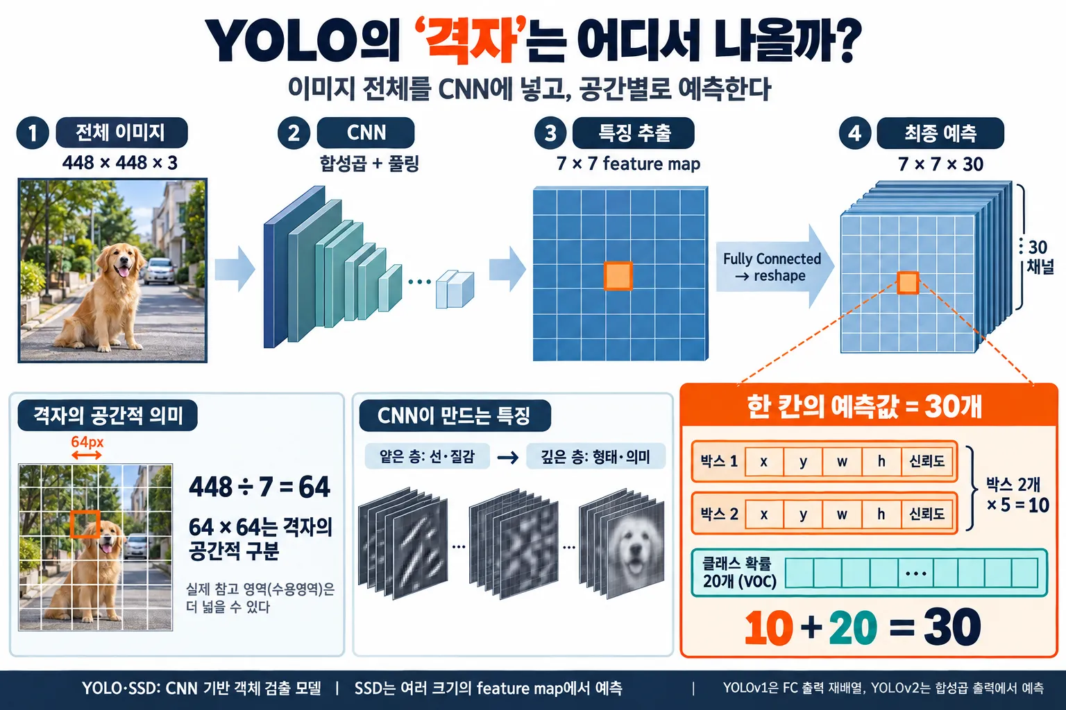
YOLO와 SSD는 모두 CNN이다. 이미지를 잘라서 넣는 게 아니라 통째로 넣고, CNN을 거쳐 나온 **feature map의 가로세로 크기가 곧 ‘격자’**다.

YOLOv1으로 보면 448×448×3 이미지가 합성곱과 풀링을 거쳐 7×7 크기의 feature map이 된다. 448 ÷ 7 = 64이므로, feature map의 한 위치는 원본 이미지의 약 64×64 픽셀 영역에 대응한다. 흔히 말하는 “한 칸”은 feature map의 한 위치이고, 그 위치에 담긴 숫자 묶음이 예측값이다.

YOLOv1의 최종 출력은 7×7×30이다. 한 칸의 숫자 30개는 박스 2개 × (x, y, w, h, 신뢰도) = 10개에 클래스 확률 20개(VOC 기준)를 더한 값이다. 엄밀히 말하면 v1은 마지막 fully connected 층의 출력을 7×7×30 모양으로 바꾼 것이고, v2부터는 합성곱 feature map을 그대로 격자로 쓴다.

CNN의 층 위치에 따라 feature map의 성격이 다르다. 이 차이가 뒤의 모든 내용을 관통한다.

	앞쪽 층	깊은 층
feature map 크기	크다 (촘촘한 격자)	작다 (성긴 격자)
한 위치의 시야	좁다	넓다
잘 아는 것	선, 질감 같은 세부 정보	“이건 새다” 같은 의미 정보
비유	시력은 좋지만 경험 없는 신입	경험은 많지만 시력이 나쁜 베테랑

YOLOv1 vs SSD300: 차이는 두 가지다

차이 1. Feature Map: 하나 vs 여러 해상도

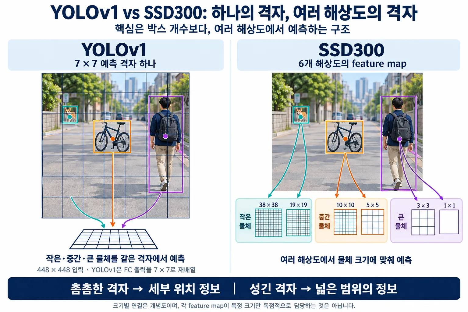
YOLOv1은 7×7 격자 하나로 모든 크기의 물체를 예측한다. SSD300은 CNN의 여러 지점에서 나온 feature map 6개를 각각 예측에 쓴다. 각 위치에는 모양이 다른 default box가 4~6개씩 놓인다.

SSD300 feature map	한 위치의 시야 (300px 기준)	위치당 default box	박스 수
38×38	약 8px	4	5,776
19×19	약 16px	6	2,166
10×10	30px	6	600
5×5	60px	6	150
3×3	100px	4	36
1×1	300px	4	4
합계			8,732

YOLOv1의 박스는 7 × 7 × 2 = 98개다. 그래서 “SSD는 박스가 많아서 작은 물체를 잘 잡는다”고 생각하기 쉽지만, 핵심은 개수가 아니다. YOLOv1의 칸당 박스를 178개로 늘려 총 8,722개로 맞춰도 작은 물체는 여전히 잘 못 잡는다. 이유는 두 가지다.

해상도: 7×7은 가장 깊은 층의 feature map이라 20px짜리 작은 물체는 이미 뭉개져 있다. 보이지 않는 물체는 박스를 아무리 많이 그려도 못 잡는다.
칸당 클래스 한 세트: v1은 한 칸에서 클래스 예측을 한 번만 한다. 작은 물체 여러 개의 중심이 한 칸에 몰리면 사실상 하나만 담당할 수 있다.

SSD는 이를 크기별 분업으로 푼다. 덜 압축된 38×38 feature map에는 작은 틀을 놓아 작은 물체를 맡기고, 시야가 넓은 3×3, 1×1에는 큰 틀을 놓아 큰 물체를 맡긴다.

차이는 박스 개수가 아니라, 여러 해상도의 격자로 물체 크기별 분업을 하느냐다.

차이 2. 박스: 처음부터 그리기 vs 틀 보정하기

사람 박스가 가로 50, 세로 150 픽셀이라고 하자.

YOLOv1: 아무 기준 없이 “가로 50, 세로 150”이라는 값 자체를 맞혀야 한다. 학습 초반에는 엉뚱한 값에서 출발한다.
SSD300: 그 자리에 이미 세로로 긴 default box(예: 60×180)가 놓여 있다. “가로 조금 줄이고, 세로 조금 줄여라” 같은 작은 보정값만 배우면 된다.

맞혀야 하는 값의 범위가 좁으니 학습이 더 안정적이다.

정리: v1의 약점 두 개와 해결 도구

v1의 약점	해결 도구	SSD	YOLO
작은 물체를 못 잡음	여러 해상도의 격자 (feature map)	처음부터 사용	v3에서 도입
박스 학습이 어려움	미리 놓인 틀	default box	v2에서 anchor 도입

SSD는 두 도구를 처음부터 갖고 나왔고, YOLO는 v2와 v3에 걸쳐 하나씩 따라잡았다.

단, SSD에도 약점이 있다. 작은 물체를 맡는 38×38은 앞쪽 층이라 위치는 잘 보지만 정체를 판단하는 의미 정보가 부족하다. 신입 혼자 판단하는 셈이다. 이 약점은 YOLOv3에서 다시 등장한다.

YOLOv2: 틀을 바꾸다

해결한 문제: v1은 박스를 틀 없이 예측해서 학습이 어려웠다.

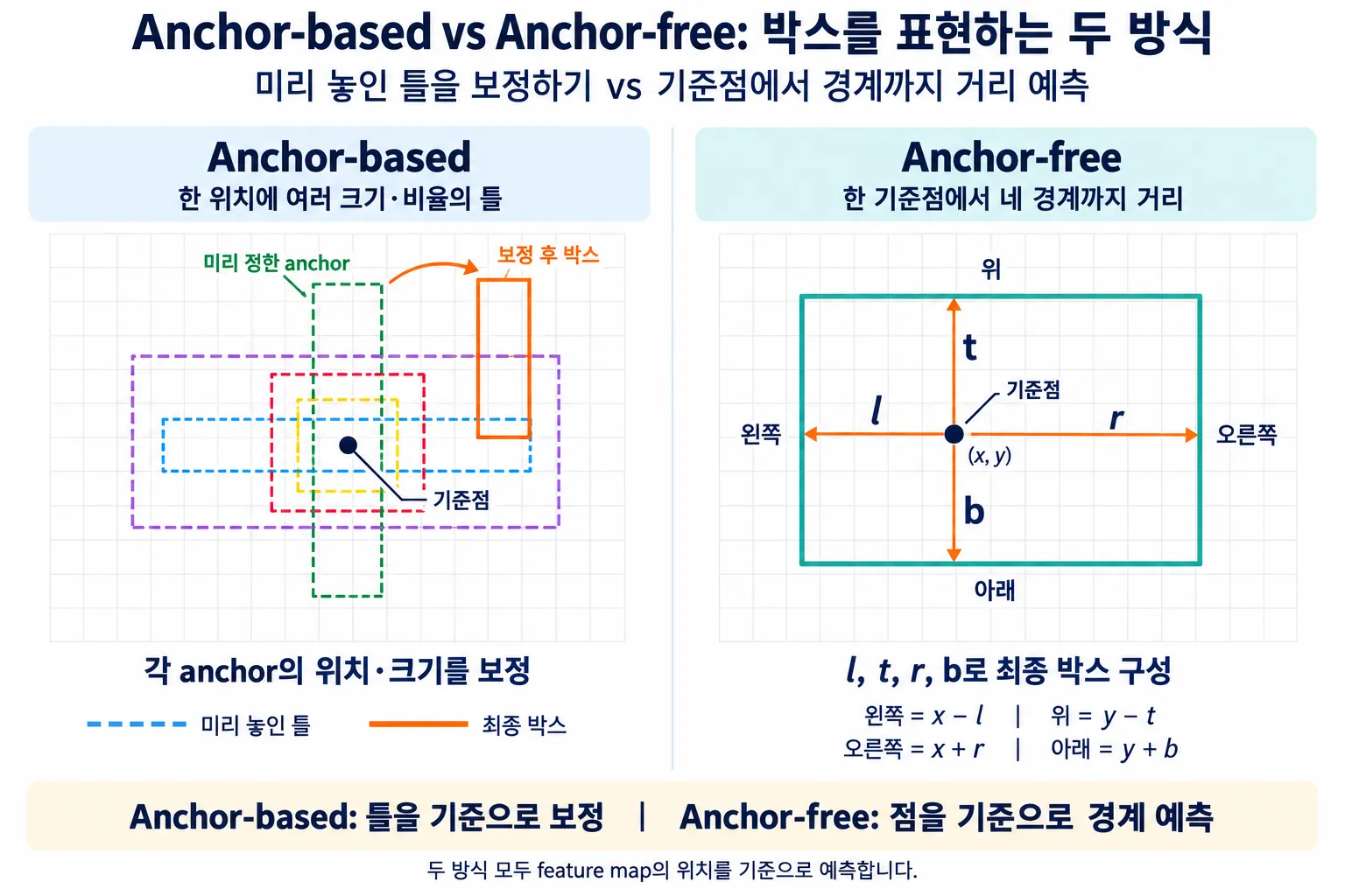
바꾼 것: k-means로 뽑은 anchor 5개를 13×13 feature map(416×416 입력 기준)의 각 칸에 놓고, 그 틀을 보정하는 값만 예측하게 했다.

SSD의 default box는 연구자가 모양을 정했다. 그런데 전봇대나 기차처럼 길쭉한 물체가 대부분인 데이터라면 미리 정한 틀이 잘 맞지 않는다. v2는 학습 데이터의 실제 박스들을 k-means로 묶어 대표 모양을 뽑았다. 이때 거리 기준으로 유클리드 거리(몇 픽셀 차이인가) 대신 1 − IoU를 썼다. 유클리드 거리를 쓰면 큰 박스는 조금만 달라도 거리가 크게 나와 불공평하기 때문이다.

칸은 한 위치지만 anchor는 그 칸을 중심으로 원본 이미지 위에 놓이는 틀이라 칸보다 훨씬 커도 된다. 지도에 꽂은 핀 하나를 중심으로 크기가 다른 원을 여러 개 그리는 것과 같다. 한 칸의 깊은 feature는 여러 번의 합성곱을 거쳐 32×32보다 훨씬 넓은 주변을 보고 만들어졌으므로 큰 박스도 판단할 수 있다.

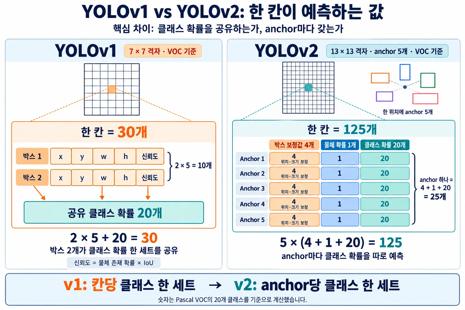
출력은 13×13×125다(VOC 기준).

anchor 하나 = 위치 보정값 4 + 물체 확률 1 + 클래스 확률 20 = 25개
칸 하나 = 25 × anchor 5개 = 125개

v1은 클래스 확률을 칸당 한 세트만 가졌지만, v2는 anchor마다 따로 가진다. 그래서 한 칸에서 사람과 자전거처럼 서로 다른 물체를 동시에 말할 수 있다.

참고로 v2도 앞쪽 26×26의 세부 정보를 끌어오는 passthrough layer를 썼지만, 예측은 여전히 13×13 한 곳에서만 했다. 격자 문제는 v3로 넘어간다.

YOLOv3: 격자를 바꾸다

해결한 문제: v2는 예측에 쓰는 feature map이 1개뿐이라 작은 물체에 약했다.

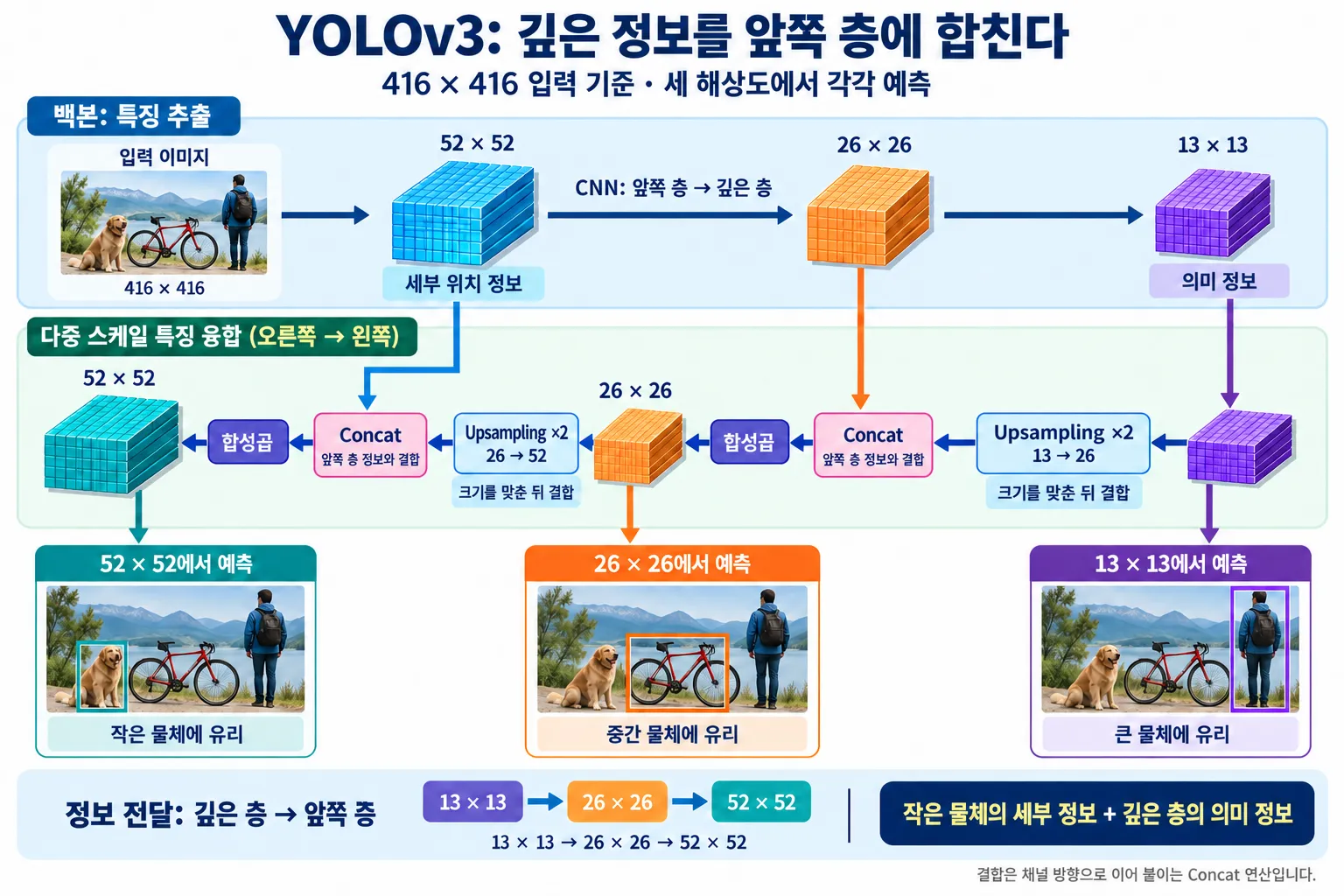
바꾼 것: 13×13, 26×26, 52×52 세 feature map에서 예측하고(416×416 입력 기준), 깊은 층의 정보를 upsampling으로 키워 앞쪽 층에 합쳤다.

anchor는 v2의 k-means 방식을 이어받아 9개를 뽑고, 크기에 맞게 격자마다 3개씩 나눠 맡긴다. SSD의 크기별 분업과 v2의 데이터 맞춤형 틀을 합친 셈이다.

여기에 SSD보다 한 걸음 더 나간 부분이 있다. SSD는 작은 물체를 앞쪽 층(신입) 혼자 판단하지만, YOLOv3는 깊은 층(베테랑)의 판단 정보를 확대해서 앞쪽 층의 세부 정보와 합쳐 예측한다. 이 구조는 FPN(Feature Pyramid Network)의 아이디어에서 왔다.

정보가 흐르는 방향은 연산의 모양으로 확인할 수 있다. upsampling은 작은 feature map을 키우는 연산이다. 13×13과 26×26을 합치려면 크기가 같아야 하므로, 깊은 층인 13×13을 두 배로 키워 26×26에 합친다. 26×26도 같은 방식으로 52×52에 합친다. 즉 정보는 깊은 층 → 앞쪽 층으로 흐른다.

YOLOv8: anchor를 버리다

해결한 문제: k-means anchor는 데이터에 갇혀 있었다. 데이터셋이 바뀔 때마다 다시 계산해야 하고, 결국 정해진 몇 개의 모양 안에서만 출발한다.

바꾼 것: anchor 없이(anchor-free), 격자의 각 점에서 물체의 왼쪽·위·오른쪽·아래 경계까지의 거리 4개를 직접 예측한다.

세 가지 해상도의 격자는 그대로 유지했다. 640×640 입력이면 80×80, 40×40, 20×20 feature map에서 예측한다. 촘촘한 80×80의 점은 작은 물체만, 성긴 20×20의 점은 큰 물체만 맡는다.

그렇다면 v1처럼 틀 없이 예측하는데 왜 학습이 어렵지 않을까? v1에도 기준점(칸)은 있었다. 차이는 기준점이 얼마나 촘촘하고, 각자 맡은 범위가 얼마나 좁으냐다. v1은 한 점이 모든 크기를 다 맡았지만, v8은 크기별 분업 덕분에 각 점이 예측하는 거리가 자기 격자 크기에 맞는 좁은 범위로 줄어든다.

v3부터 이어진 크기별 격자 분업이 “대략 이 정도 크기”라는 출발점을 대신해 주기 때문에, v8은 데이터마다 다시 맞춰야 하는 anchor 없이도 각 점에서 경계까지의 거리를 안정적으로 학습할 수 있다.

주의할 점이 두 가지 있다.

YOLO 계열에서 anchor-free를 처음 시도한 것은 v8이 아니라 YOLOX(2021)다.
v8은 anchor-free 외에도 여러 부분을 동시에 바꿨다. 그래서 “anchor를 버려서 성능이 좋아졌다”고 단정할 수는 없다. “구조가 더 단순해졌다”가 정확한 표현이다.

YOLOv10 / YOLO26: NMS를 버리다

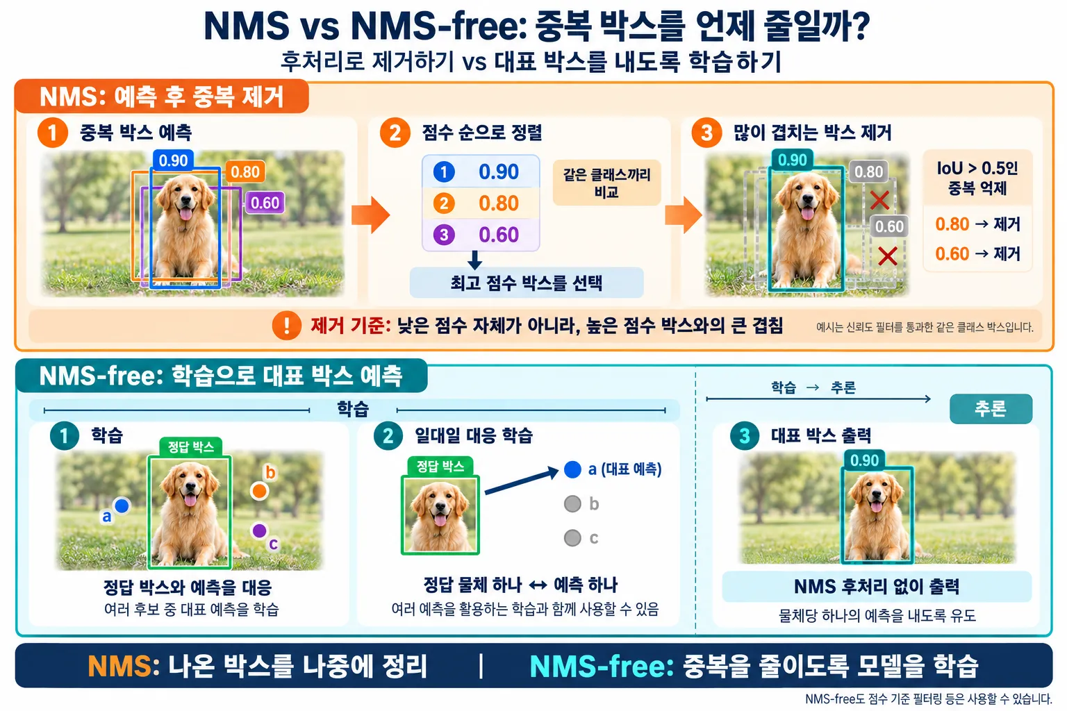
해결한 문제: NMS는 바짝 붙은 같은 클래스 물체 중 하나를 지울 수 있고, 모델 밖의 별도 후처리라 느리다.

바꾼 것: 중복 박스를 나중에 지우는 대신, 처음부터 물체 하나당 박스 하나만 내도록 모델을 훈련해서 NMS를 없앴다.

NMS는 어떻게 동작하나

신뢰도 필터 (NMS 전): 점수가 기준값(예: 0.25)보다 낮은 박스를 버린다.
정렬: 남은 박스를 클래스별로 점수 순으로 줄 세운다.
억제: 1등 박스와 IoU가 기준값(예: 0.5)보다 큰 박스를 지운다. 남은 박스 중 다시 1등을 뽑아 반복한다.

점수는 “누가 대표가 될지”를, IoU는 “누가 그 대표의 중복인지”를 정한다. 박스는 점수가 낮아서가 아니라 나보다 점수 높은 박스와 많이 겹쳐서 지워진다. 예를 들어 같은 고양이에 점수 0.9, 0.8, 0.3인 박스가 있을 때, 0.9와 IoU 0.7로 겹친 0.8은 지워지고, IoU 0.1인 0.3은 다른 물체로 보고 남는다.

NMS의 약점

밀집한 물체: 어깨동무한 두 사람의 박스 점수가 0.9, 0.85이고 IoU가 0.6이면, 기준값 0.5에서 실제로 존재하는 두 번째 사람이 사라진다. 기준값을 0.7로 올리면 이번엔 중복 박스가 살아남는다. 데이터마다 사람이 적당한 값을 찾아야 한다는 점에서 anchor와 같은 구조의 문제다.
속도와 배포: 박스를 하나씩 비교하며 반복하므로 박스가 많을수록 느려지고, 엣지 기기에 모델을 올릴 때 걸림돌이 된다.

NMS-free

YOLOv10은 학습할 때 “물체 하나에 여러 점이 답하는 방식”과 “물체 하나에 가장 좋은 점 하나만 답하는 방식”을 함께 학습하고, 추론할 때는 후자만 써서 NMS를 없앴다.

Ultralytics가 2026년 1월 공개한 YOLO26도 이 방향을 잇는다. Ultralytics 로드맵에 따르면 YOLO26 논문은 NMS-free end-to-end 구조와 MuSGD라는 새 옵티마이저를 핵심으로 다룬다. 2026년 9월 YOLO Vision 2026 행사에서는 차세대 YOLO27이 발표됐지만, 공식 GitHub 기준으로 아직 모델은 공개되지 않았다.

한눈에 정리

YOLO의 발전은 “이전 버전의 약점을 하나씩 해결한 과정”으로 읽으면 하나의 이야기가 된다.

버전	이전의 문제	바꾼 것	바꾼 대상
YOLOv1	(출발점)	7×7 feature map 하나에서 칸마다 박스 2개를 틀 없이 예측	—
SSD300	YOLOv1의 두 약점	6개 feature map으로 크기별 분업 + default box 보정	격자, 틀
YOLOv2	박스를 틀 없이 예측해 학습이 어려움	k-means(1 − IoU)로 뽑은 anchor 5개를 보정	틀
YOLOv3	예측 feature map이 1개라 작은 물체에 약함	3개 feature map + 깊은 층 정보를 앞쪽 층에 합침(FPN식)	격자
YOLOv8	anchor가 데이터에 갇힘	anchor-free, 각 점에서 경계까지 거리 예측	틀 제거
YOLOv10 / YOLO26	NMS가 밀집 물체를 지우고 느림	물체 하나당 박스 하나로 훈련, NMS 제거	후처리 제거

어떤 구조가 약점이었는지 판단하는 기준은 하나다. 이후 버전들이 그 구조를 유지했으면 성공한 아이디어, 버렸으면 약점이다. 여러 해상도의 격자는 v3 이후 지금까지 유지됐고, anchor와 NMS는 결국 버려졌다.

참고자료

공식 문서

Introduction

SSD300 and YOLO are both 1-stage detectors that find objects by looking at the image only once. In the end, their differences come down to two things: how many grids they use and at what resolution, and whether they draw boxes from scratch or adjust pre-placed templates.

This post compares SSD300 and YOLOv1 along these two axes, then follows which weakness of the previous version each YOLO release, from v1 to YOLO26, fixed and how. It assumes you already know basic object detection concepts such as bounding boxes and IoU.

Basics: a grid is a feature map

YOLO and SSD are both CNNs. The image is not cut into pieces; it goes in whole, and the width and height of the feature map that comes out of the CNN is the “grid”.

Take YOLOv1: a 448×448×3 image becomes a 7×7 feature map after convolutions and pooling. Since 448 ÷ 7 = 64, one position in the feature map corresponds to roughly a 64×64-pixel region of the original image. What people call “one cell” is one position in the feature map, and the bundle of numbers at that position is the prediction.

YOLOv1’s final output is 7×7×30. The 30 numbers in a cell are 2 boxes × (x, y, w, h, confidence) = 10, plus 20 class probabilities (for VOC). Strictly speaking, v1 reshapes the output of its last fully connected layer into 7×7×30; from v2 on, the convolutional feature map is used directly as the grid.

Feature maps behave differently depending on where they come from in the CNN. This difference runs through everything that follows.

	Early layers	Deep layers
Feature map size	Large (dense grid)	Small (sparse grid)
Field of view per position	Narrow	Wide
Good at	Details like edges and textures	Semantic information like “this is a bird”
Analogy	A rookie with sharp eyes but no experience	A veteran with lots of experience but poor eyesight

YOLOv1 vs SSD300: there are two differences

Difference 1. Feature maps: one vs several resolutions

YOLOv1 predicts objects of every size from a single 7×7 grid. SSD300 uses six feature maps taken from different points in the CNN, each for its own predictions. Each position holds 4–6 default boxes of different shapes.

SSD300 feature map	Field of view per position (300px input)	Default boxes per position	Boxes
38×38	~8px	4	5,776
19×19	~16px	6	2,166
10×10	30px	6	600
5×5	60px	6	150
3×3	100px	4	36
1×1	300px	4	4
Total			8,732

YOLOv1 has 7 × 7 × 2 = 98 boxes. So it is tempting to think “SSD catches small objects well because it has many boxes”, but the count is not the point. Even if you raised YOLOv1 to 178 boxes per cell for a total of 8,722, it would still struggle with small objects. There are two reasons.

Resolution: 7×7 is the feature map of the deepest layer, so a small 20px object has already been smeared out. You cannot catch an object you cannot see, no matter how many boxes you draw.
One set of classes per cell: v1 predicts classes only once per cell. If the centers of several small objects fall into one cell, it can effectively handle only one of them.

SSD solves this with division of labor by size. Small templates on the less-compressed 38×38 feature map handle small objects, while large templates on the wide-view 3×3 and 1×1 maps handle large objects.

The difference is not the number of boxes but whether grids at multiple resolutions split the work by object size.

Difference 2. Boxes: drawing from scratch vs adjusting templates

Say a person’s box is 50 pixels wide and 150 pixels tall.

YOLOv1: has to hit the values “50 wide, 150 tall” themselves, with no reference point. Early in training it starts from arbitrary values.
SSD300: a tall default box (e.g. 60×180) is already sitting there. It only has to learn small corrections like “shrink the width a bit, shrink the height a bit”.

Because the range of values to predict is narrower, training is more stable.

Summary: v1’s two weaknesses and the tools that fix them

v1’s weakness	Fix	SSD	YOLO
Misses small objects	Grids at multiple resolutions (feature maps)	From the start	Introduced in v3
Box learning is hard	Pre-placed templates	Default boxes	Anchors introduced in v2

SSD came out with both tools from the start, and YOLO caught up one at a time across v2 and v3.

SSD has a weakness too, though. The 38×38 map that handles small objects comes from an early layer, so it sees position well but lacks the semantic information needed to decide what the object is. It is like leaving the rookie to judge alone. This weakness comes up again in YOLOv3.

YOLOv2: changing the templates

Problem solved: v1 predicted boxes without templates, which made training hard.

What changed: it placed 5 anchors chosen by k-means in every cell of a 13×13 feature map (for a 416×416 input), and predicted only corrections to those templates.

SSD’s default boxes had shapes chosen by the researchers. But if most objects in your data are long and thin, like utility poles or trains, predefined templates don’t fit well. v2 clustered the real boxes in the training data with k-means to pick representative shapes. As the distance it used 1 − IoU instead of Euclidean distance (how many pixels apart). With Euclidean distance, large boxes get a big distance even when they differ only slightly, which is unfair.

A cell is one position, but an anchor is a template placed on the original image centered on that cell, so it can be much larger than the cell. It is like drawing several circles of different sizes around a single pin stuck in a map. The deep feature of a cell was built from a region much wider than 32×32 through many convolutions, so it can judge large boxes too.

The output is 13×13×125 (for VOC).

One anchor = 4 position corrections + 1 objectness + 20 class probabilities = 25
One cell = 25 × 5 anchors = 125

v1 had only one set of class probabilities per cell, but v2 has one per anchor. So a single cell can talk about different objects at once, such as a person and a bicycle.

For reference, v2 also used a passthrough layer that brought in details from the earlier 26×26 map, but it still predicted from only one place, the 13×13 map. The grid problem carries over to v3.

YOLOv3: changing the grid

Problem solved: v2 used only one feature map for prediction, so it was weak on small objects.

What changed: it predicts from three feature maps, 13×13, 26×26 and 52×52 (for a 416×416 input), and merges information from deep layers into earlier layers by upsampling it.

It keeps v2’s k-means approach to pick 9 anchors and assigns 3 to each grid according to size. It effectively combines SSD’s division of labor by size with v2’s data-fitted templates.

There is also a part where it goes one step beyond SSD. SSD leaves small objects to the early layer (the rookie) alone, but YOLOv3 enlarges the judgment of the deep layer (the veteran) and combines it with the early layer’s details to make its predictions. This structure comes from the idea behind FPN (Feature Pyramid Network).

You can see which way information flows from the shape of the operations. Upsampling enlarges a small feature map. To merge 13×13 with 26×26 they must be the same size, so the deep 13×13 map is doubled and merged into 26×26. 26×26 is merged into 52×52 the same way. In other words, information flows from deep layers → to early layers.

YOLOv8: dropping anchors

Problem solved: k-means anchors were trapped in the data. They had to be recomputed whenever the dataset changed, and predictions still started from only a fixed handful of shapes.

What changed: without anchors (anchor-free), each grid point directly predicts four distances to the object’s left, top, right and bottom edges.

It kept the grids at three resolutions. For a 640×640 input it predicts from 80×80, 40×40 and 20×20 feature maps. Points on the dense 80×80 grid handle only small objects, and points on the sparse 20×20 grid handle only large ones.

So why isn’t training hard, if it predicts without templates like v1? v1 had reference points (cells) too. The difference is how dense the reference points are and how narrow each one’s range is. In v1 one point handled every size, but in v8, thanks to the division of labor by size, the distances each point predicts shrink to a narrow range that matches its grid size.

The size-based grid split that started in v3 stands in for the “roughly this big” starting point, so v8 can learn the distance from each point to the edges stably without anchors that have to be refitted for every dataset.

Two caveats:

The first anchor-free attempt in the YOLO family was not v8 but YOLOX (2021).
v8 changed many parts at once besides going anchor-free. So you cannot conclude that “dropping anchors improved performance”. “The architecture became simpler” is the accurate way to put it.

YOLOv10 / YOLO26: dropping NMS

Problem solved: NMS can delete one of two tightly packed objects of the same class, and it is slow because it is separate post-processing outside the model.

What changed: instead of removing duplicate boxes afterwards, the model is trained from the start to output only one box per object, eliminating NMS.

How NMS works

Confidence filter (before NMS): discard boxes whose score is below a threshold (e.g. 0.25).
Sort: line up the remaining boxes by score within each class.
Suppress: delete boxes whose IoU with the top box exceeds a threshold (e.g. 0.5). Pick the top box among the rest and repeat.

The score decides “who becomes the representative”, and IoU decides “who is a duplicate of that representative”. A box is deleted not because its score is low, but because it overlaps heavily with a box that scores higher. For example, if the same cat has boxes scoring 0.9, 0.8 and 0.3, the 0.8 box that overlaps the 0.9 box at IoU 0.7 is deleted, while the 0.3 box at IoU 0.1 is treated as a different object and kept.

NMS’s weaknesses

Crowded objects: if two people with arms around each other have boxes scoring 0.9 and 0.85 with an IoU of 0.6, a threshold of 0.5 makes the second person, who really exists, disappear. Raise the threshold to 0.7 and duplicate boxes survive instead. Having a person find the right value for every dataset is the same kind of problem as anchors.
Speed and deployment: it compares boxes one by one in a loop, so it gets slower as boxes increase and becomes an obstacle when deploying models to edge devices.

NMS-free

During training, YOLOv10 learns both “several points answer for one object” and “only the single best point answers for one object”, and at inference it uses only the latter, eliminating NMS.

YOLO26, released by Ultralytics in January 2026, continues in this direction. According to the Ultralytics roadmap, the YOLO26 paper centers on an NMS-free end-to-end architecture and a new optimizer called MuSGD. The next-generation YOLO27 was announced at the YOLO Vision 2026 event in September 2026, but as of the official GitHub the model has not been released yet.

Summary at a glance

Read as “a process of fixing the previous version’s weaknesses one at a time”, YOLO’s evolution becomes a single story.

Version	Previous problem	What changed	What was changed
YOLOv1	(starting point)	Predicts 2 boxes per cell without templates from one 7×7 feature map	—
SSD300	YOLOv1’s two weaknesses	Division of labor by size across 6 feature maps + default box corrections	Grid, templates
YOLOv2	Predicting boxes without templates made training hard	Corrects 5 anchors chosen by k-means (1 − IoU)	Templates
YOLOv3	One prediction feature map, weak on small objects	3 feature maps + merging deep-layer information into early layers (FPN-style)	Grid
YOLOv8	Anchors trapped in the data	Anchor-free, predicts distances from each point to the edges	Templates removed
YOLOv10 / YOLO26	NMS deletes crowded objects and is slow	Trained for one box per object, NMS removed	Post-processing removed

There is one rule for deciding which structure was a weakness: if later versions kept a structure, it was a successful idea; if they dropped it, it was a weakness. Grids at multiple resolutions have been kept from v3 to today, while anchors and NMS were eventually dropped.

References

Official documentation

References

- Liu et al., “SSD: Single Shot MultiBox Detector”, ECCV 2016 (arXiv 1512.02325)
- Redmon et al., “You Only Look Once: Unified, Real-Time Object Detection”, CVPR 2016 (arXiv 1506.02640)
- Redmon & Farhadi, “YOLO9000: Better, Faster, Stronger”, CVPR 2017 (arXiv 1612.08242)
- Redmon & Farhadi, “YOLOv3: An Incremental Improvement”, 2018 (arXiv 1804.02767)
- Lin et al., “Feature Pyramid Networks for Object Detection”, CVPR 2017 (arXiv 1612.03144)
- Ge et al., “YOLOX: Exceeding YOLO Series in 2021” (arXiv 2107.08430)
- Wang et al., “YOLOv10: Real-Time End-to-End Object Detection”, 2024 (arXiv 2405.14458)