축구 경기 Semantic Segmentation에서 클래스 불균형 다루기 (U-Net++)Handling Class Imbalance in Soccer Semantic Segmentation (U-Net++)
문제 정의: 이미지 세그멘테이션에서 클래스 불균형은 어떻게 해결해야 할까?
축구 중계 화면 100장으로 픽셀 단위 분할 모델을 학습시키면서, 픽셀 비율 1%도 안 되는 작은 클래스(공, 심판, 골키퍼 B) 가 왜 잘 안 잡히는지, 원인이 무엇인지 실험으로 좁혀 간 기록입니다.
한 줄 요약
- BCE + Dice로 학습한 U-Net++는 평균 성능은 괜찮았지만 작은 클래스가 fold에 따라 IoU 0 ↔ 0.8로 갈렸다.
- 시드만 바꿔도 결과가 갈리는 것을 확인 → 원인은 데이터 분할이 아니라 작은 클래스의 학습 불안정.
- CE + Dice + 클래스 가중치로 바꾸자 test mIoU 0.770 → 0.873, Ball IoU 0 → 0.771.
1. 데이터셋
- Football Semantic Segmentation (Acme AI, Kaggle)
- 2017 UEFA 슈퍼컵 레알 마드리드 vs 맨체스터 유나이티드 하이라이트에서 12프레임마다 뽑은 100장 (1920×1080)
- COCO 폴리곤 어노테이션 915개, 11개 클래스
- Team A / Team B / Goalkeeper A / Goalkeeper B / Referee / Coaches & Officials
- Ball / Goal Bar / Ground / Audience / Advertisement
Coaches & Officials는 어노테이션이 0건이라 제외 → 실제 학습 클래스는 10개, 배경 클래스 없음 (모든 픽셀에 라벨 존재)
2. 데이터 확인 – 학습 전에 확인한 것들
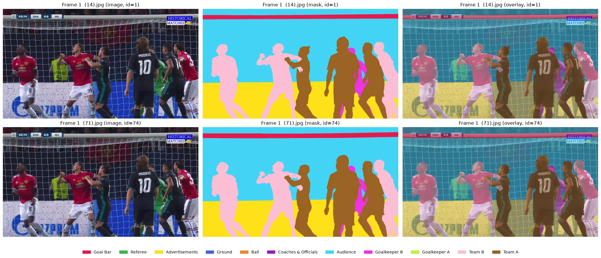
2.1. 완전 중복 이미지 (MD5)
파일명은 다르지만 내용이 완전히 같은 이미지가 1쌍 있었습니다. (Frame 1 (14), Frame 1 (71))
이 둘이 train과 test로 갈리면 사실상 정답을 보고 시험을 보는 셈이라, 분할할 때 같은 쪽에 묶어야 합니다.
2.2. 유사 이미지 (pHash)
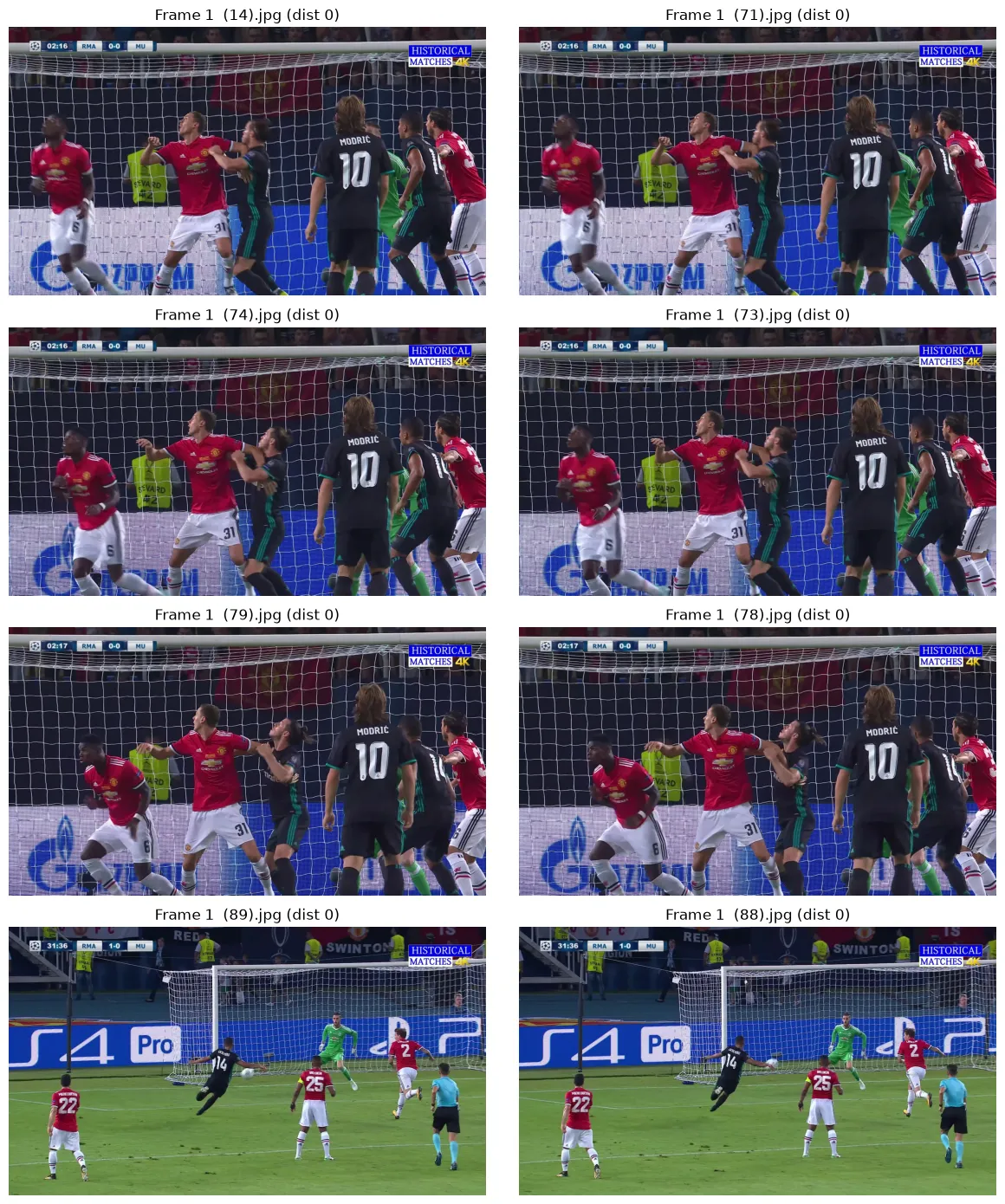
영상에서 프레임을 뽑은 데이터라 “똑같진 않지만 거의 같은” 장면이 많을 것이라 생각했고, pHash(64bit, 해밍거리 ≤ 5)로 검사했습니다.
- 유사 이미지 32장 / 100장, 8개 그룹 (최대 그룹 10장)
- 데이터의 1/3이 서로 닮은 프레임이라, 무작위로 나누면 val/test 점수가 부풀려질 위험이 큼
→ 유사 그룹은 전부 train에 고정하고, 나머지에서 val/test를 뽑았습니다.
2.3. 클래스 비율 – 인스턴스 수 vs 픽셀 면적
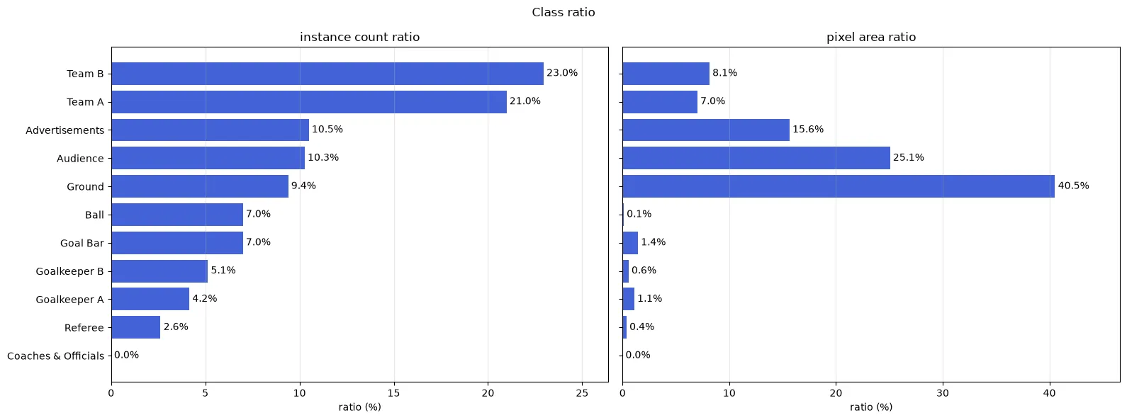
데이터셋 문서(PDF)에 적힌 클래스 비율은 인스턴스 수 기준입니다. 그런데 세그멘테이션 손실은 픽셀 단위로 계산되니, 픽셀 면적 기준으로 다시 봤습니다.
| 클래스 | 인스턴스 비율 | 픽셀 면적 비율 |
|---|---|---|
| Ground | 9.4% | 40.5% |
| Audience | 10.3% | 25.1% |
| Ball | 7.0% | 0.1% |
| Referee | 2.6% | 0.4% |
| Goalkeeper B | 5.1% | 0.6% |
인스턴스 수로 보면 Ball이 7%로 꽤 있어 보이지만, 픽셀로는 0.1% 입니다. Ground와는 400배 차이. 이 프로젝트의 핵심 문제가 여기서 드러났습니다.
그 외 확인한 것:
- 사람(선수/골키퍼/심판)이 없는 이미지: 0장 (이미지당 평균 5.1명)
- 마스크 좌표가 이미지 밖으로 나간 경우: 0건 (폴리곤 2,397개 검사)
2.4. train / val / test 분할
- 70 / 15 / 15장
- 유사 이미지 32장은 train 고정
- 나머지에서 인스턴스 수·픽셀 면적·등장 이미지 수 세 가지 비율이 모두 7:1.5:1.5에 가깝도록 탐색해서 분할 (편차 점수 0.094)
3. 전처리 / 증강
| 변환 | 설정 | 마스크에도 적용 |
|---|---|---|
| RandomResizedCrop | scale 0.4~1.0, 출력 576×1024 | O (nearest) |
| HorizontalFlip | p=0.5 | O |
| ColorJitter | 밝기/대비/채도 0.3 | X |
| GaussianBlur | p=0.2 | X |
| Normalize | ImageNet 평균/표준편차 (ResNet34 백본) | X |
- 입력 크기 576×1024: 원본과 같은 16:9, 32의 배수
- 라벨맵은 큰 객체부터 칠해서 작은 객체(공 등)가 위에 덮이도록 함
4. LAB 1 – U-Net++ + BCE + Dice
4.1. 모델
U-Net++ (encoder: ImageNet 사전학습 ResNet34)
U-Net은 디코더가 인코더의 같은 층 피처맵 하나만 스킵 커넥션으로 받지만, U-Net++는 인코더-디코더 사이에 중간 노드를 두고 각 노드가 같은 층의 앞선 노드들을 전부 이어붙입니다 (DenseNet 아이디어). 인코더와 디코더 피처 사이의 의미 차이(semantic gap)를 줄이는 구조입니다.
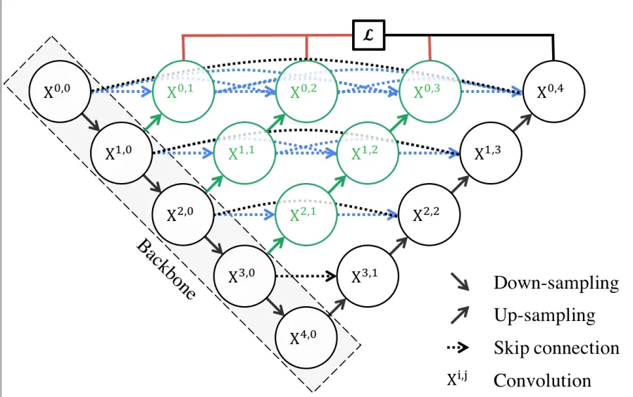 출처: Zhou et al., UNet++ (2018)
- 손실: BCE + Dice (클래스별 sigmoid)
- 지표: mIoU, mDice, mAP, 경계 지표(Boundary F1, Boundary IoU)
- 사전학습 encoder는 lr 1e-4, 새로 만든 decoder는 1e-3
4.2. 학습 결과
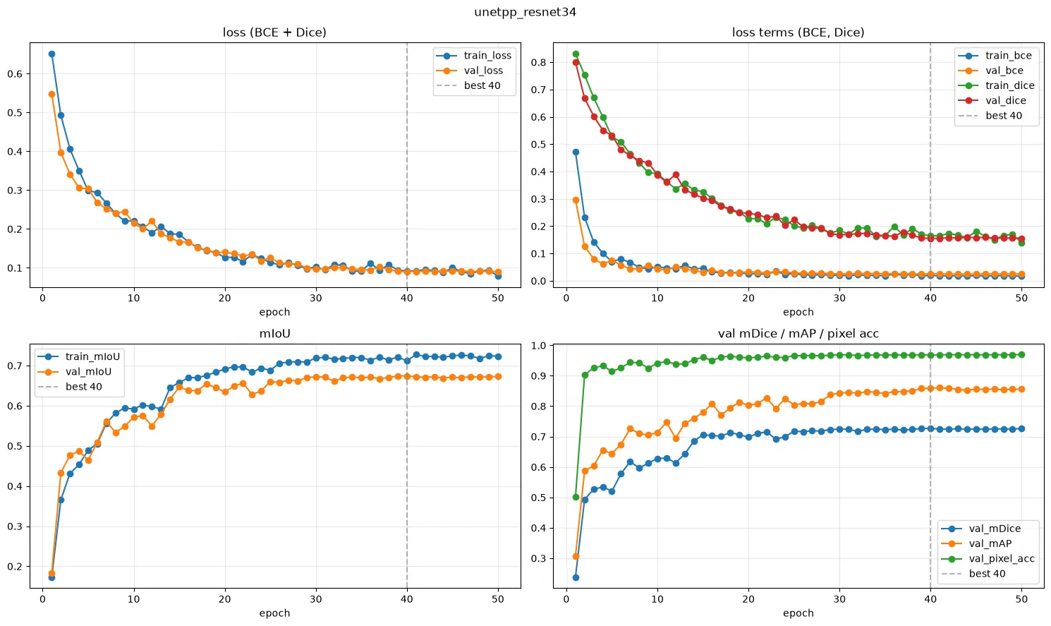
- best epoch 40, val mIoU 0.674, mDice 0.727, mAP 0.859
- train/val loss가 함께 내려가 과적합은 크지 않음
- 다만 mAP(0.86)에 비해 mIoU·mDice가 눈에 띄게 낮음 → 점수 순위는 맞게 매기는데 최종 판정(argmax)에서 틀리는 클래스가 있다는 신호
4.3. 5-Fold 교차검증
val 15장은 너무 적어서, 이 점수가 믿을 만한지 확인하려고 train+val 85장으로 5-Fold를 돌렸습니다. (test는 손대지 않음, 유사 그룹은 한 fold에 통째로)
| fold | mIoU | mDice | mAP | best epoch |
|---|---|---|---|---|
| 1 | 0.645 | 0.698 | 0.732 | 14 |
| 2 | 0.664 | 0.711 | 0.864 | 44 |
| 3 | 0.792 | 0.841 | 0.951 | 49 |
| 4 | 0.884 | 0.937 | 0.958 | 50 |
| 5 | 0.780 | 0.832 | 0.922 | 41 |
| 평균 | 0.753 ± 0.099 | 0.804 ± 0.100 | 0.886 ± 0.093 |
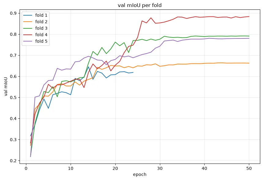
fold 간 mIoU 차이가 0.645 ~ 0.884로 너무 큽니다.
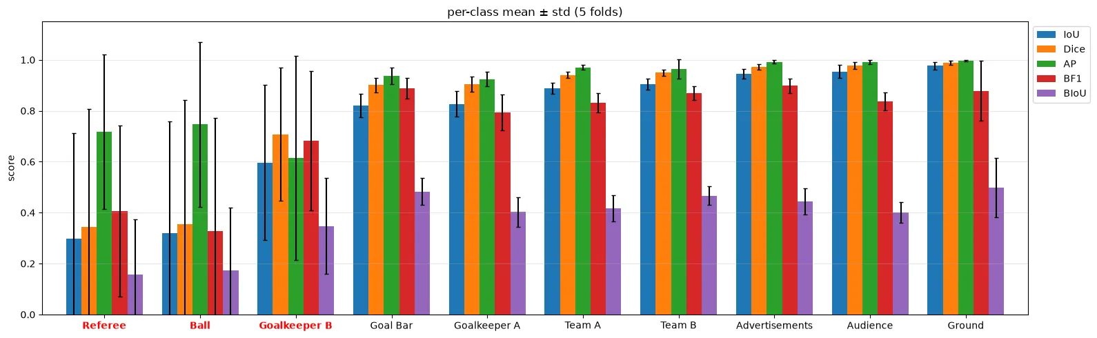
클래스별로 쪼개 보면 원인이 바로 보입니다. 막대는 5-fold 평균, 수염은 표준편차입니다.
| 클래스 | 픽셀 비율 | IoU (mean ± std) | AP (mean ± std) |
|---|---|---|---|
| Ground | 40.1% | 0.976 ± 0.016 | 0.997 |
| Audience | 25.3% | 0.954 ± 0.026 | 0.991 |
| Team B | 8.3% | 0.905 ± 0.022 | 0.965 |
| Goalkeeper B | 0.56% | 0.596 ± 0.304 | 0.615 |
| Referee | 0.37% | 0.299 ± 0.412 | 0.717 |
| Ball | 0.11% | 0.320 ± 0.438 | 0.746 |
큰 클래스는 0.9 이상으로 안정적인데, 픽셀 1% 미만인 3개 클래스만 표준편차가 0.3~0.44로 요동칩니다. fold별 IoU를 보면 더 극단적입니다.
| fold 1 | fold 2 | fold 3 | fold 4 | fold 5 | |
|---|---|---|---|---|---|
| Ball | 0.000 | 0.000 | 0.780 | 0.819 | 0.000 |
| Referee | 0.010 | 0.000 | 0.000 | 0.850 | 0.634 |
| Goalkeeper B | 0.235 | 0.309 | 0.879 | 0.852 | 0.707 |
“조금 못 잡는다”가 아니라 아예 못 잡거나(0) 꽤 잘 잡거나(0.8) 둘 중 하나입니다.
4.4. 못 잡은 객체를 직접 보기
val에서 recall이 가장 낮은 객체를 확대해서 봤습니다. (초록 = 맞힘, 빨강 = 놓침)
Ball – 10개 중 10개 모두 놓침 (recall 0)
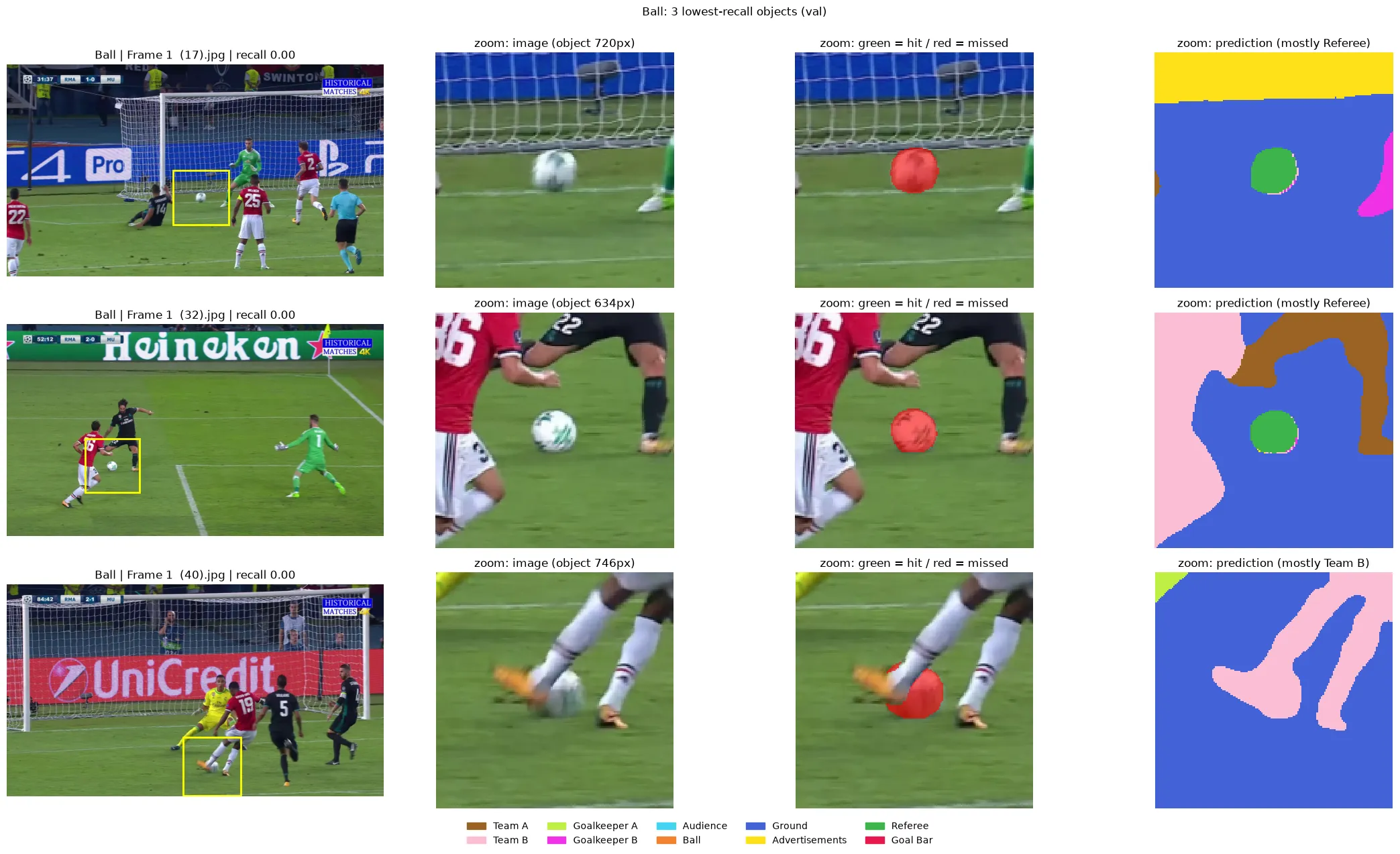
- 공의 면적은 중앙값 720px (576×1024 입력에서 0.1%)
- 놓친 공의 74%를 Referee로 예측
- 그런데 AP는 0.7 이상 → 모델이 공 픽셀에 “공일 가능성”을 어느 정도는 주지만, argmax에서 더 큰 클래스에 진다
Goalkeeper B – 주로 Team A로 혼동 (32%)
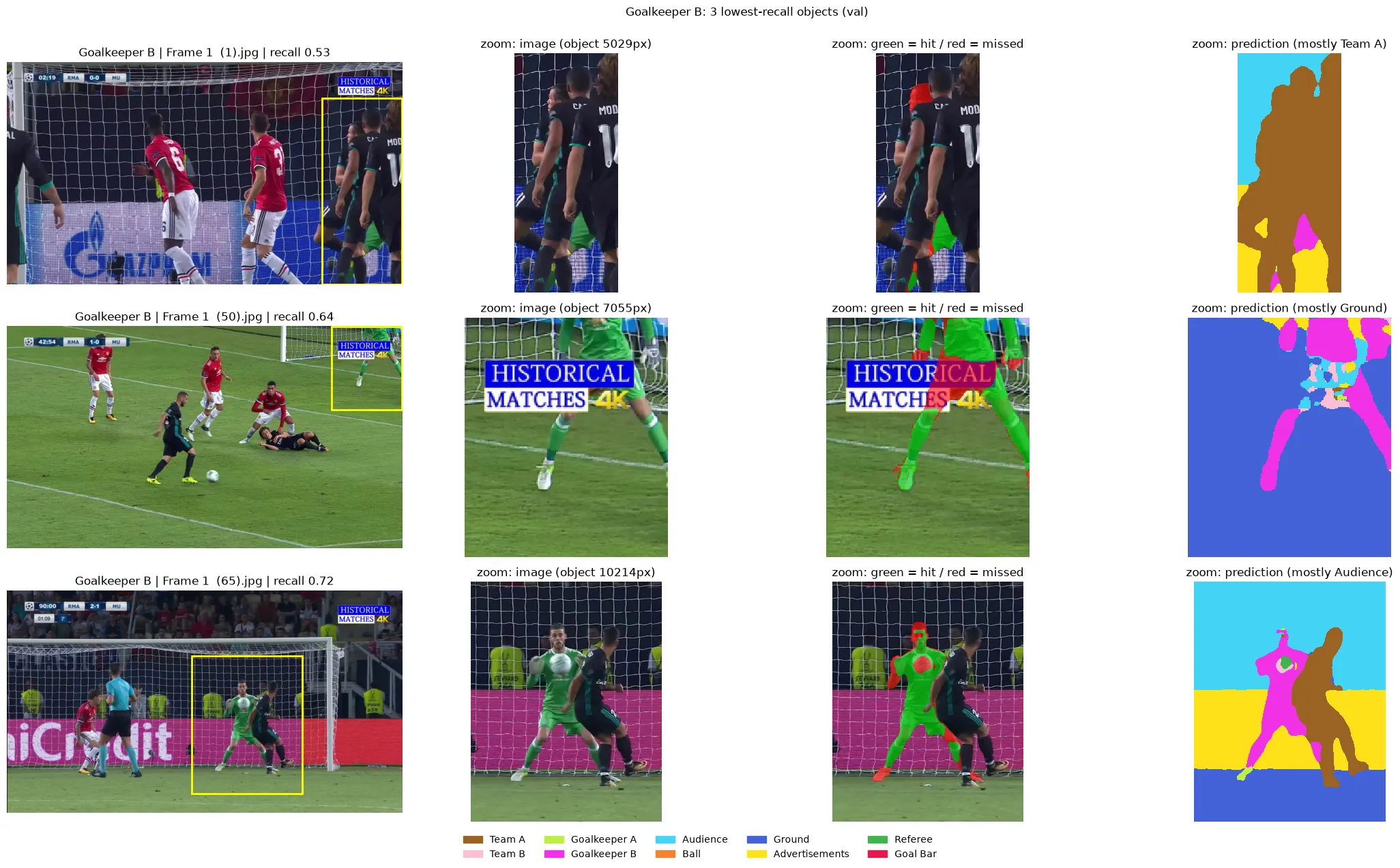
선수와 겹쳐 있거나, 중계 화면 로고에 가려진 경우에 다른 선수 클래스로 흡수됐습니다.
4.5. 가설 세우기
작은 클래스가 fold에 따라 0 또는 0.8로 갈리는 이유로 두 가지를 생각했습니다.
- fold별 train 구성 차이 – 어떤 fold는 train에 작은 클래스 예시가 부족해서
- 작은 클래스의 학습 불안정 – 손실에서 차지하는 비중이 너무 작아 늦게, 불안정하게 학습돼서
실제로 fold 분할 결과를 보면 Referee는 fold 2에 35%가 몰려 있었고(목표 20%), Ball이 있는 이미지 수도 fold 1만 7장(나머지 11~12장)이라 가설 ①도 충분히 그럴듯했습니다.
5. LAB 2 – 시드만 바꿔 보기
두 가설을 구분하는 가장 간단한 방법은 train 구성은 그대로 두고 시드만 바꾸는 것입니다.
- 결과가 비슷하다 → 가설 ① (데이터 구성 문제)
- 결과가 크게 갈린다 → 가설 ② (학습 자체가 불안정)
fold 2(base mIoU 0.664)에서 시드 42 / 43 / 44로 다시 학습했습니다.
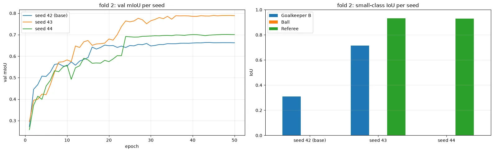
| 시드 | mIoU | Goalkeeper B | Ball | Referee |
|---|---|---|---|---|
| 42 (base) | 0.664 | 0.309 | 0.000 | 0.000 |
| 43 | 0.790 | 0.713 | 0.000 | 0.933 |
| 44 | 0.701 | 0.002 | 0.000 | 0.930 |
같은 데이터인데 Goalkeeper B는 0.002 ~ 0.713, Referee는 0 ~ 0.933으로 흔들립니다. → 가설 ② 쪽. 데이터 분할이 아니라 작은 클래스가 학습 자체에서 불안정하다는 것. (Ball은 세 시드 모두 0이라, 이 손실 설정으로는 아예 학습이 안 되고 있었습니다.)
6. LAB 3 – CE + Dice + 클래스 가중치
학습 불안정이 원인이라면, 손실 함수에서 작은 클래스의 목소리를 키워야 합니다. 두 가지를 바꿨습니다.
- BCE → CE (softmax) BCE는 클래스마다 독립적인 “있다/없다” 문제로 풀어서, 픽셀 하나에 정답이 하나인 이 데이터와 맞지 않습니다. CE는 클래스끼리 직접 경쟁시키므로 argmax 판정과 학습 목표가 일치합니다.
- 클래스 가중치 (픽셀 빈도에 반비례)
| 클래스 | 가중치 |
|---|---|
| Ball | 3.36 |
| Referee | 1.78 |
| Goalkeeper B | 1.48 |
| Goalkeeper A | 1.02 |
| Team A / B | 0.41 / 0.39 |
| Audience | 0.22 |
| Ground | 0.17 |
5개 fold 모두 같은 분할·같은 시드로 다시 학습했습니다. (점선 = BCE + Dice, 실선 = CE + Dice + 가중치)
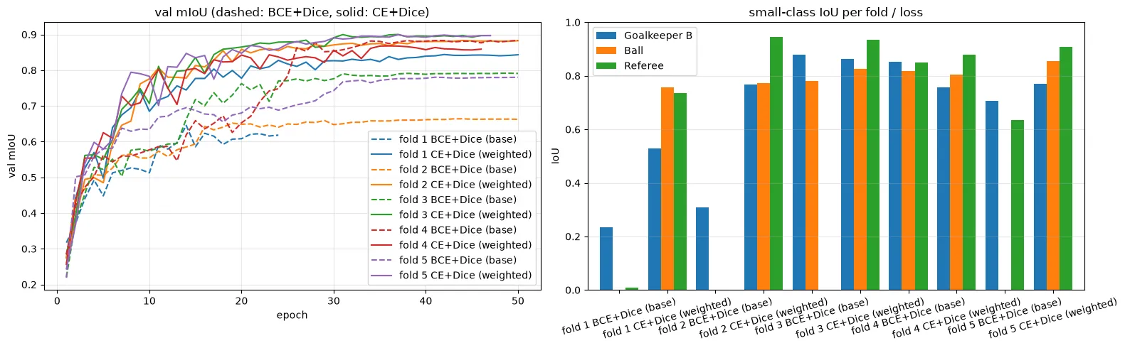
| fold | BCE+Dice mIoU | CE+Dice(w) mIoU | Ball | Referee | Goalkeeper B |
|---|---|---|---|---|---|
| 1 | 0.645 | 0.844 | 0 → 0.756 | 0.010 → 0.736 | 0.235 → 0.529 |
| 2 | 0.664 | 0.883 | 0 → 0.773 | 0 → 0.946 | 0.309 → 0.768 |
| 3 | 0.792 | 0.900 | 0.780 → 0.827 | 0 → 0.934 | 0.879 → 0.864 |
| 4 | 0.884 | 0.868 | 0.819 → 0.805 | 0.850 → 0.880 | 0.852 → 0.757 |
| 5 | 0.780 | 0.899 | 0 → 0.856 | 0.634 → 0.907 | 0.707 → 0.769 |
| 평균 | 0.753 ± 0.099 | 0.879 ± 0.024 |
- 평균 mIoU +0.126
- fold 간 표준편차 0.099 → 0.024 (약 1/4)
- IoU 0이던 칸이 모두 사라짐
- 큰 클래스(Ground, Audience, Advertisements)의 변화는 ±0.01 수준으로 거의 그대로
mAP는 이 비교에서 뺐습니다. AP를 sigmoid(logit)로 계산하는데, softmax로 학습한 CE 모델의 logit은 sigmoid 확률처럼 보정돼 있지 않아 BCE 모델과 공정하게 비교하기 어렵기 때문입니다.
7. 최종 test 평가
test 15장은 학습과 모델 선택에 한 번도 쓰지 않았고, 딱 한 번만 평가했습니다. CE + Dice 모델은 val mIoU가 가장 높은 fold 3 모델을 사용했습니다.
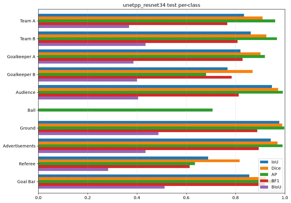
BCE + Dice (가중치 X) – Ball 막대가 AP(초록)만 남고 IoU/Dice는 0
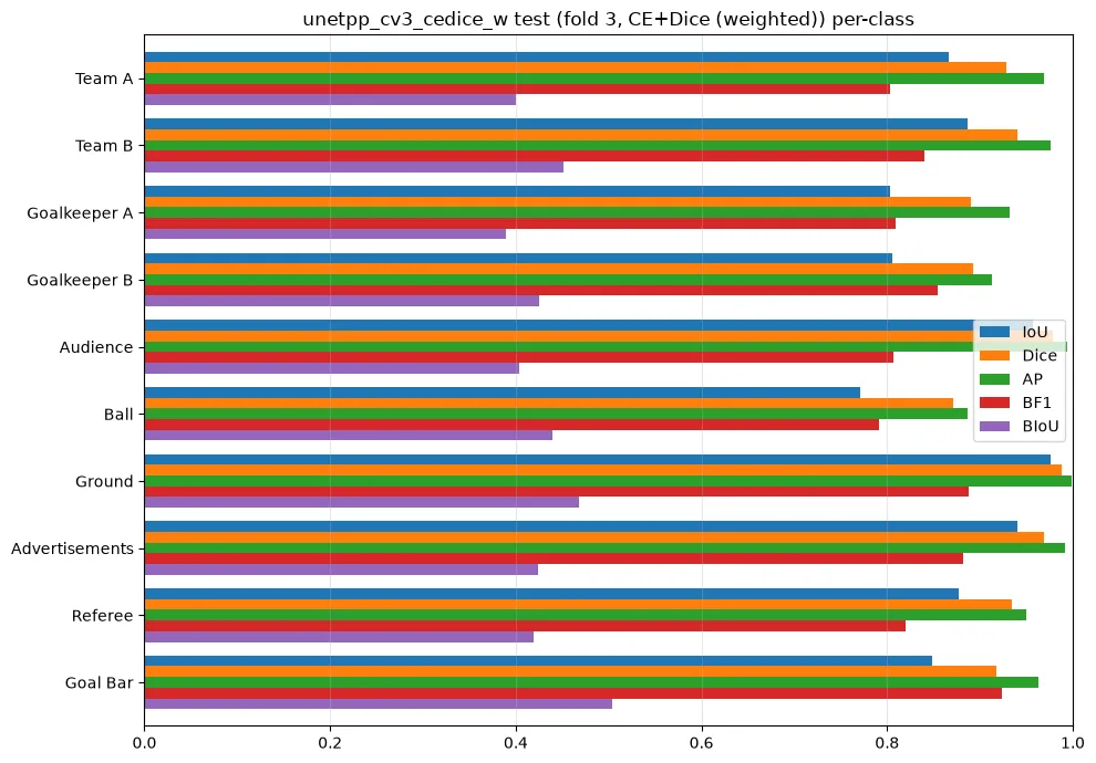
CE + Dice + 클래스 가중치 – 모든 클래스가 고르게
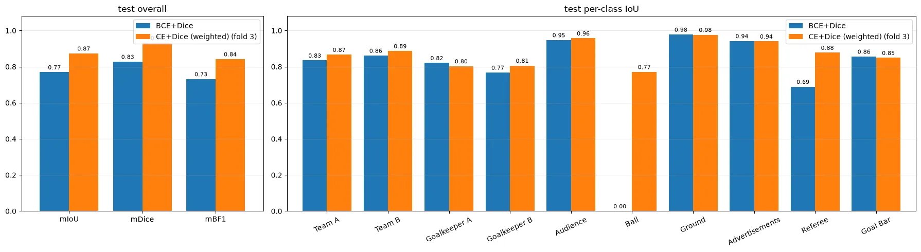
| 모델 | mIoU | mDice | mBF1 | Goalkeeper B | Ball | Referee |
|---|---|---|---|---|---|---|
| BCE + Dice | 0.770 | 0.828 | 0.731 | 0.767 | 0.000 | 0.689 |
| CE + Dice + 가중치 | 0.873 | 0.931 | 0.842 | 0.806 | 0.771 | 0.878 |
- BCE + Dice는 test에서도 공을 하나도 못 잡았습니다 (AP는 0.71인데 IoU 0)
- CE + Dice + 가중치는 Ball IoU를 0 → 0.771로 올렸고, 큰 클래스 성능은 유지
- 사람 클래스(Team A/B, Goalkeeper A/B, Referee) test IoU가 모두 0.80 ~ 0.89로 고르게 나옴
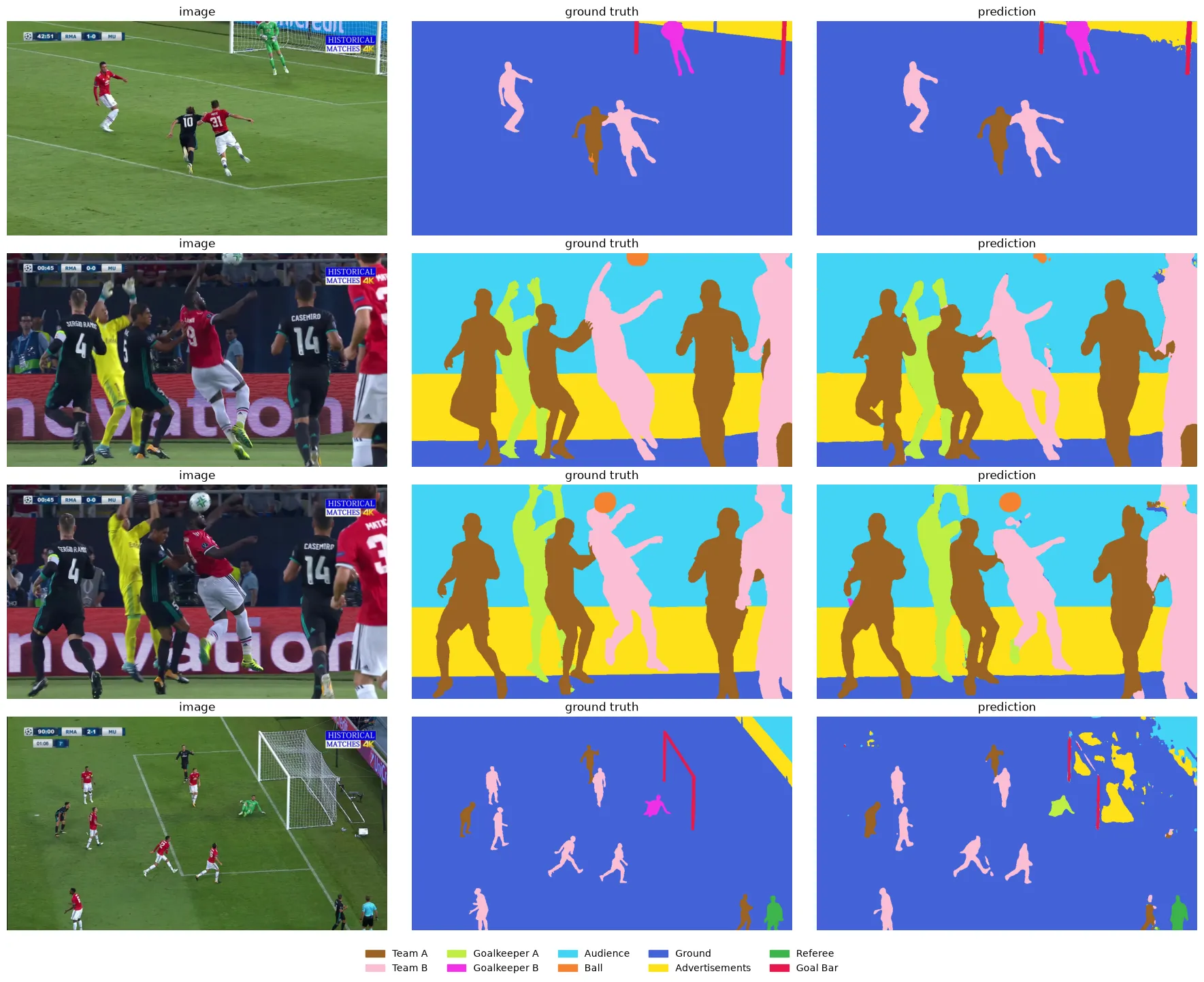
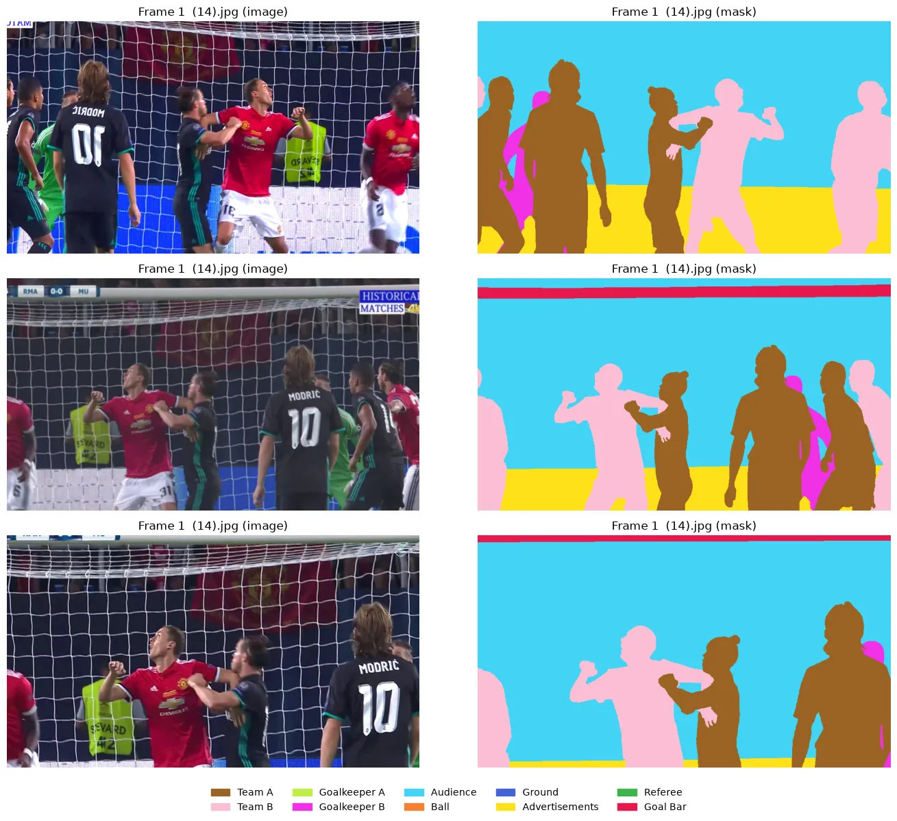
왼쪽부터 원본 / 정답 / 예측 (CE + Dice + 가중치)
8. 결론
- 작은 클래스 성능이 fold마다 0 ↔ 0.8로 갈린 원인은 데이터 분할이 아니라, 작은 클래스가 손실에서 차지하는 비중이 작아 학습이 불안정한 것이었다. (시드만 바꿔도 결과가 갈림)
- “AP는 높은데 IoU는 0” 이라는 패턴이 결정적인 단서였다. 모델이 작은 클래스를 아예 모르는 게 아니라, argmax 경쟁에서 큰 클래스에 밀리고 있었던 것.
- 손실을 CE + Dice + 클래스 가중치로 바꾸자 평균은 오르고(+0.126) 편차는 1/4로 줄었다.
- 데이터 확인 단계에서 인스턴스 비율이 아니라 픽셀 비율을 본 것이 문제를 빨리 짚는 데 도움이 됐다.
9. 한계와 다음 단계
- 두 가지를 동시에 바꿨다. LAB 3에서 BCE → CE와 클래스 가중치를 함께 바꿔서, 각각의 기여도는 분리하지 못했다. → CE + Dice(가중치 X), BCE + Dice(가중치 O)를 따로 돌려 비교할 예정
- test 비교의 두 모델은 학습 데이터 구성이 완전히 같지 않다. (BCE: train 70장 / CE: fold 3의 68장)
- 시드 비교 3개, test 15장으로 신뢰구간이 넓다. → 시드와 데이터를 늘릴 필요
- 경계 지표 mBIoU가 0.43으로 아직 낮다. 윤곽을 정확히 따야 한다면 경계 손실이나 고해상도 입력을 검토
- 실제 중계 카메라 추적에 쓰려면 연속 프레임에서의 안정성과 추론 속도도 확인해야 한다.
Problem: how should class imbalance be handled in image segmentation?
This is a record of training a pixel-level segmentation model on 100 soccer broadcast frames, and narrowing down through experiments why small classes that make up less than 1% of pixels (ball, referee, goalkeeper B) were so hard to detect, and what the cause was.
TL;DR
- U-Net++ trained with BCE + Dice had decent average performance, but small classes swung between IoU 0 and 0.8 depending on the fold.
- Results diverged even when only the seed changed → the cause was not the data split but unstable learning of small classes.
- Switching to CE + Dice + class weights raised test mIoU from 0.770 → 0.873 and Ball IoU from 0 → 0.771.
1. Dataset
- Football Semantic Segmentation (Acme AI, Kaggle)
- 100 frames (1920×1080) sampled every 12 frames from highlights of the 2017 UEFA Super Cup, Real Madrid vs Manchester United
- 915 COCO polygon annotations, 11 classes
- Team A / Team B / Goalkeeper A / Goalkeeper B / Referee / Coaches & Officials
- Ball / Goal Bar / Ground / Audience / Advertisement
Coaches & Officialshas zero annotations and was excluded → 10 classes actually trained, no background class (every pixel has a label)
2. Looking at the data – what I checked before training
2.1. Exact duplicate images (MD5)
There was one pair of images with different file names but identical content (Frame 1 (14), Frame 1 (71)).
If they ended up split across train and test, it would be like taking an exam after seeing the answers, so they have to be kept on the same side when splitting.
2.2. Near-duplicate images (pHash)
Since the frames were extracted from video, I expected many scenes that are “not identical but nearly the same”, and checked them with pHash (64-bit, Hamming distance ≤ 5).
- 32 of 100 images were near-duplicates, in 8 groups (largest group: 10 images)
- With a third of the data being look-alike frames, a random split carries a high risk of inflating val/test scores
→ All near-duplicate groups were fixed to train, and val/test were drawn from the rest.
2.3. Class ratios – instance count vs pixel area
The class ratios in the dataset’s documentation (PDF) are by instance count. But the segmentation loss is computed per pixel, so I looked again by pixel area.
| Class | Instance ratio | Pixel area ratio |
|---|---|---|
| Ground | 9.4% | 40.5% |
| Audience | 10.3% | 25.1% |
| Ball | 7.0% | 0.1% |
| Referee | 2.6% | 0.4% |
| Goalkeeper B | 5.1% | 0.6% |
By instance count the ball looks fairly common at 7%, but by pixels it is 0.1% — 400 times less than Ground. This is where the core problem of the project showed up.
Other checks:
- Images with no people (players/goalkeepers/referee): 0 (5.1 people per image on average)
- Mask coordinates outside the image: 0 cases (2,397 polygons checked)
2.4. train / val / test split
- 70 / 15 / 15 images
- The 32 near-duplicate images fixed to train
- From the rest, searched for a split where instance count, pixel area and number of images containing each class were all close to 7:1.5:1.5 (deviation score 0.094)
3. Preprocessing / augmentation
| Transform | Settings | Applied to mask too |
|---|---|---|
| RandomResizedCrop | scale 0.4–1.0, output 576×1024 | O (nearest) |
| HorizontalFlip | p=0.5 | O |
| ColorJitter | brightness/contrast/saturation 0.3 | X |
| GaussianBlur | p=0.2 | X |
| Normalize | ImageNet mean/std (ResNet34 backbone) | X |
- Input size 576×1024: the same 16:9 as the original, and a multiple of 32
- The label map was painted from the largest objects first so small objects (like the ball) end up on top
4. LAB 1 – U-Net++ + BCE + Dice
4.1. Model
U-Net++ (encoder: ResNet34 pretrained on ImageNet)
In U-Net, the decoder receives only one feature map from the same level of the encoder through a skip connection. U-Net++ places intermediate nodes between the encoder and decoder, and each node concatenates all of the earlier nodes at the same level (the DenseNet idea). The structure reduces the semantic gap between encoder and decoder features.
Source: Zhou et al., UNet++ (2018)
- Loss: BCE + Dice (per-class sigmoid)
- Metrics: mIoU, mDice, mAP, boundary metrics (Boundary F1, Boundary IoU)
- Pretrained encoder at lr 1e-4, newly built decoder at 1e-3
4.2. Training results
- Best epoch 40, val mIoU 0.674, mDice 0.727, mAP 0.859
- Train and val loss went down together, so overfitting was not large
- However, mIoU and mDice were noticeably lower than mAP (0.86) → a sign that the model ranks scores correctly but some classes lose at the final decision (argmax)
4.3. 5-fold cross-validation
15 val images are too few, so to check whether this score could be trusted I ran 5-fold on the 85 train+val images. (Test untouched; each near-duplicate group kept whole within one fold.)
| fold | mIoU | mDice | mAP | best epoch |
|---|---|---|---|---|
| 1 | 0.645 | 0.698 | 0.732 | 14 |
| 2 | 0.664 | 0.711 | 0.864 | 44 |
| 3 | 0.792 | 0.841 | 0.951 | 49 |
| 4 | 0.884 | 0.937 | 0.958 | 50 |
| 5 | 0.780 | 0.832 | 0.922 | 41 |
| Mean | 0.753 ± 0.099 | 0.804 ± 0.100 | 0.886 ± 0.093 |
The mIoU gap between folds, 0.645 – 0.884, is far too large.
Breaking it down by class shows the cause right away. Bars are the 5-fold mean, whiskers the standard deviation.
| Class | Pixel ratio | IoU (mean ± std) | AP (mean ± std) |
|---|---|---|---|
| Ground | 40.1% | 0.976 ± 0.016 | 0.997 |
| Audience | 25.3% | 0.954 ± 0.026 | 0.991 |
| Team B | 8.3% | 0.905 ± 0.022 | 0.965 |
| Goalkeeper B | 0.56% | 0.596 ± 0.304 | 0.615 |
| Referee | 0.37% | 0.299 ± 0.412 | 0.717 |
| Ball | 0.11% | 0.320 ± 0.438 | 0.746 |
The large classes are stable above 0.9, but only the three classes under 1% of pixels swing with a standard deviation of 0.3–0.44. Per-fold IoU is even more extreme.
| fold 1 | fold 2 | fold 3 | fold 4 | fold 5 | |
|---|---|---|---|---|---|
| Ball | 0.000 | 0.000 | 0.780 | 0.819 | 0.000 |
| Referee | 0.010 | 0.000 | 0.000 | 0.850 | 0.634 |
| Goalkeeper B | 0.235 | 0.309 | 0.879 | 0.852 | 0.707 |
It is not “detects them a little poorly” but either not at all (0) or fairly well (0.8).
4.4. Looking at the missed objects directly
I zoomed in on the objects with the lowest recall in val. (Green = hit, red = missed)
Ball – missed all 10 of 10 (recall 0)
- Median ball area is 720px (0.1% of a 576×1024 input)
- 74% of missed balls were predicted as Referee
- Yet AP is above 0.7 → the model does give ball pixels some “probability of being the ball”, but loses to a larger class at argmax
Goalkeeper B – mostly confused with Team A (32%)
When overlapping with other players or hidden behind the broadcast logo, they were absorbed into another player class.
4.5. Forming hypotheses
I considered two reasons why small classes split between 0 and 0.8 depending on the fold.
- Different train composition per fold – some folds lack small-class examples in train
- Unstable learning of small classes – their share of the loss is so small that they are learned late and unstably
Looking at the actual fold split, 35% of Referee was concentrated in fold 2 (target 20%), and only fold 1 had 7 images containing the ball (the others had 11–12), so hypothesis ① was quite plausible too.
5. LAB 2 – changing only the seed
The simplest way to tell the two hypotheses apart is to keep the train composition the same and change only the seed.
- Results are similar → hypothesis ① (a data composition problem)
- Results diverge a lot → hypothesis ② (training itself is unstable)
I retrained fold 2 (base mIoU 0.664) with seeds 42 / 43 / 44.
| Seed | mIoU | Goalkeeper B | Ball | Referee |
|---|---|---|---|---|
| 42 (base) | 0.664 | 0.309 | 0.000 | 0.000 |
| 43 | 0.790 | 0.713 | 0.000 | 0.933 |
| 44 | 0.701 | 0.002 | 0.000 | 0.930 |
With the same data, Goalkeeper B swings from 0.002 to 0.713 and Referee from 0 to 0.933. → Hypothesis ②. It is not the data split; the small classes are unstable in the training itself. (Ball was 0 for all three seeds, so with this loss setup it was not being learned at all.)
6. LAB 3 – CE + Dice + class weights
If unstable training is the cause, the loss function has to amplify the voice of the small classes. I changed two things.
- BCE → CE (softmax) BCE treats each class as an independent “present / absent” problem, which does not fit this data where each pixel has exactly one answer. CE makes the classes compete directly, so the training objective matches the argmax decision.
- Class weights (inversely proportional to pixel frequency)
| Class | Weight |
|---|---|
| Ball | 3.36 |
| Referee | 1.78 |
| Goalkeeper B | 1.48 |
| Goalkeeper A | 1.02 |
| Team A / B | 0.41 / 0.39 |
| Audience | 0.22 |
| Ground | 0.17 |
All 5 folds were retrained with the same splits and the same seed. (Dashed = BCE + Dice, solid = CE + Dice + weights)
| fold | BCE+Dice mIoU | CE+Dice(w) mIoU | Ball | Referee | Goalkeeper B |
|---|---|---|---|---|---|
| 1 | 0.645 | 0.844 | 0 → 0.756 | 0.010 → 0.736 | 0.235 → 0.529 |
| 2 | 0.664 | 0.883 | 0 → 0.773 | 0 → 0.946 | 0.309 → 0.768 |
| 3 | 0.792 | 0.900 | 0.780 → 0.827 | 0 → 0.934 | 0.879 → 0.864 |
| 4 | 0.884 | 0.868 | 0.819 → 0.805 | 0.850 → 0.880 | 0.852 → 0.757 |
| 5 | 0.780 | 0.899 | 0 → 0.856 | 0.634 → 0.907 | 0.707 → 0.769 |
| Mean | 0.753 ± 0.099 | 0.879 ± 0.024 |
- Mean mIoU +0.126
- Standard deviation across folds 0.099 → 0.024 (about 1/4)
- Every cell that had IoU 0 disappeared
- Large classes (Ground, Audience, Advertisements) changed by only about ±0.01, nearly unchanged
I left mAP out of this comparison. AP is computed from sigmoid(logit), and the logits of a CE model trained with softmax are not calibrated like sigmoid probabilities, so a fair comparison with the BCE model is difficult.
7. Final test evaluation
The 15 test images were never used for training or model selection, and were evaluated exactly once. For CE + Dice, I used the fold 3 model, which had the highest val mIoU.
BCE + Dice (no weights) – the Ball bar has only AP (green); IoU/Dice are 0
CE + Dice + class weights – all classes even
| Model | mIoU | mDice | mBF1 | Goalkeeper B | Ball | Referee |
|---|---|---|---|---|---|---|
| BCE + Dice | 0.770 | 0.828 | 0.731 | 0.767 | 0.000 | 0.689 |
| CE + Dice + weights | 0.873 | 0.931 | 0.842 | 0.806 | 0.771 | 0.878 |
- BCE + Dice did not catch a single ball on test either (AP 0.71 but IoU 0)
- CE + Dice + weights raised Ball IoU from 0 → 0.771 while keeping performance on the large classes
- Test IoU for the person classes (Team A/B, Goalkeeper A/B, Referee) came out evenly at 0.80 – 0.89
From left: original / ground truth / prediction (CE + Dice + weights)
8. Conclusion
- The reason small-class performance split between 0 and 0.8 across folds was not the data split but unstable training, because small classes make up so little of the loss. (Results diverged just by changing the seed.)
- The pattern “high AP but IoU 0” was the decisive clue. The model did not know nothing about the small classes; it was losing the argmax competition to the large ones.
- Switching the loss to CE + Dice + class weights raised the mean (+0.126) and cut the variance to 1/4.
- Looking at pixel ratios rather than instance ratios during the data check helped pinpoint the problem quickly.
9. Limitations and next steps
- I changed two things at once. LAB 3 switched BCE → CE and added class weights together, so the contribution of each could not be separated. → Plan to run CE + Dice (no weights) and BCE + Dice (with weights) separately and compare
- The two models in the test comparison were not trained on exactly the same data. (BCE: 70 train images / CE: 68 images from fold 3)
- With only 3 seeds compared and 15 test images, confidence intervals are wide. → More seeds and more data are needed
- The boundary metric mBIoU is still low at 0.43. If contours need to be precise, consider a boundary loss or higher-resolution input
- To use this for tracking with real broadcast cameras, stability across consecutive frames and inference speed also need to be checked.