제약이 능력을 만든다: PyTorch로 이해하는 AE, DAE, VAEConstraints Create Capability: Understanding AE, DAE and VAE with PyTorch
오토인코더를 처음 접하면 목표부터 이상하게 느껴진다. 입력한 이미지를 그대로 출력하도록 학습한다니, return x 한 줄이면 끝나는 것 아닐까?
하지만 입력이 좁은 통로를 지나야 한다면 이야기가 달라진다. 784개 픽셀을 더 적은 수의 값으로 표현하고 다시 복원하려면, 어떤 특징을 남길지 학습해야 한다.
이번 글에서는 MNIST 손글씨 이미지로 세 가지 모델을 살펴본다.
| 모델 | 학습 방식 | 살펴볼 질문 |
|---|---|---|
| AE · Autoencoder | 입력을 압축한 뒤 복원 | 작은 잠재 벡터에 무엇이 남을까? |
| DAE · Denoising Autoencoder | 손상된 입력에서 원본 복원 | 노이즈를 넣으면 무엇을 배우게 될까? |
| VAE · Variational Autoencoder | 이미지별 잠재 분포로 복원하고 기준 분포에 가깝게 유도 | 새 이미지를 만들 좌표는 어디서 뽑을까? |
아래 수치와 그림은 실습 노트북에 저장된 실행 결과다. 모델 초기화, 난수, 실행 환경에 따라 재실행 결과는 달라질 수 있다. 본문에는 핵심 코드를 싣고, 긴 비교·시각화 코드는 마지막 부록에 모았다.
1. 실습 준비: 28×28 이미지를 784차원 벡터로
MNIST 이미지는 28×28 크기의 흑백 이미지다. ToTensor()로 픽셀을 0~1 범위의 텐서로 바꾸고, 완전연결층에 넣기 전에 784차원으로 펼친다.
필요한 패키지는 다음과 같이 설치한다.
pip install torch torchvision matplotlib다음은 원본 실습의 환경 설정이다. Apple Silicon의 MPS를 사용할 수 있으면 활용하고, 그렇지 않으면 CPU에서 실행한다.
import torch
import torch.nn as nn
import torch.nn.functional as F
from torch.utils.data import DataLoader
from torchvision import datasets, transforms
import matplotlib.pyplot as plt

# 모델 초기화와 노이즈 생성 등에 사용할 공통 시드입니다.
SEED = 42
torch.manual_seed(SEED)

device = "mps" if torch.backends.mps.is_available() else "cpu"

train_set = datasets.MNIST("./data", train=True, download=True,
                           transform=transforms.ToTensor())
train_loader = DataLoader(train_set, batch_size=256, shuffle=True)DataLoader는 학습 데이터를 256장씩 묶어 제공한다. 한 번에 처리하는 양과 업데이트 횟수를 조절하기 위한 선택이다.
torch.flatten(images, start_dim=1)은 배치 차원을 유지하면서 이미지 차원만 합친다.
[배치 크기, 1, 28, 28] → [배치 크기, 784]2. AE: 복원을 배우게 하는 병목
AE는 인코더와 디코더로 구성된다.
- 인코더: 입력
x를 잠재 벡터z로 변환한다. - 디코더: 잠재 벡터
z로 복원 이미지x̂를 만든다.
이번 모델의 구조는 다음과 같다.
입력 784 → 은닉층 128 → 잠재 벡터 32 → 은닉층 128 → 출력 784잠재 벡터는 이미지를 복원하는 데 사용할 요약 표현이다. 병목은 정보를 그대로 전달하기 어렵게 만들지만, 사람이 원하는 의미적 특징을 자동으로 보장하지는 않는다.
class AutoEncoder(nn.Module):
    #잠재표현 층을 몇 차원으로 줄건지 latent_dim으로 받음.
    def __init__(self, latent_dim):
        super().__init__()
        #encoder
        self.encoder = nn.Sequential(
            nn.Linear(784, 128),
            nn.ReLU(),
            nn.Linear(128, latent_dim)
        )
        #decoder
        self.decoder = nn.Sequential(
            nn.Linear(latent_dim, 128),
            nn.ReLU(),
            nn.Linear(128, 784),
            nn.Sigmoid()
        )
    #forward = 순전파
    def forward(self, x):
        z = self.encoder(x)
        return self.decoder(z)
마지막 Sigmoid는 출력 픽셀을 0~1 범위로 제한한다. forward()에서는 입력을 인코딩한 뒤 바로 디코딩한다.
숫자 레이블 대신 입력 자체를 목표로 사용한다
학습할 때 숫자 클래스 레이블은 사용하지 않는다. 대신 복원 결과와 입력 이미지 사이의 MSE, 즉 픽셀별 평균 제곱 오차를 줄인다.
여기서 “레이블을 쓰지 않는다”는 “학습 목표가 없다”는 뜻이 아니다. 입력 이미지 자체가 복원의 목표다. MSE는 이번 실습에서 선택한 복원 손실이며, 픽셀이 연속값이라는 이유로 반드시 MSE만 써야 하는 것은 아니다.
model = AutoEncoder(latent_dim=32).to(device)
criterion = nn.MSELoss()
optimizer = torch.optim.Adam(model.parameters(), lr=1e-3)

for epoch in range(5):
    total = 0
    for images, _ in train_loader:
        #start_dim=1: 1번 차원부터 합치기를 시작합니다. (보통 0번 차원은 배치 크기(Batch Size)이므로 유지합니다.)
        x = torch.flatten(images, start_dim=1).to(device)

        output = model(x)
        loss = criterion(output, x)

        optimizer.zero_grad()
        loss.backward()
        optimizer.step()

        total += loss.item()
    print(f"epoch {epoch+1}: {total/len(train_loader):.4f}")
저장된 학습 로그는 다음과 같다. 이 값은 각 epoch의 배치별 평균 손실을 다시 평균한 학습 지표다.
epoch 1: 0.0645
epoch 2: 0.0304
epoch 3: 0.0210
epoch 4: 0.0172
epoch 5: 0.0151
손실은 감소했다. 실제 복원 이미지도 확인해보자.
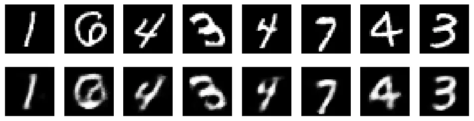
위: 원본 이미지 · 아래: 잠재 차원 32인 AE의 복원 결과. 학습 데이터에서 뽑은 예시다.
잠재 차원을 784로 늘리면 완벽하게 복사할까?
현재 모델에서는 잠재 차원만 늘려도 다음 구조가 된다.
784 → 128 → 784 → 128 → 784여전히 128차원 층이 남아 있다. 따라서 잠재 차원이 입력과 같아졌다는 이유만으로 병목이 없어졌다고 말할 수 없다.
중간 층까지 넓히고 구조와 활성화 함수가 허용하면 항등 함수를 표현할 수 있지만, 학습이 실제로 그 해에 도달하는지는 별개의 문제다. 또 처음 보는 입력까지 그대로 반환하는 항등 함수와 훈련 데이터만 외우는 과적합도 구분해야 한다.
핵심은 복원을 잘하는 것과 다른 작업에도 유용한 표현을 배우는 것은 서로 다른 평가 대상이라는 점이다.
3. 잠재 차원을 줄이면 무엇을 잃을까?
잠재 차원을 2, 4, 8, 16, 32, 64로 바꾸어 비교했다. 모든 모델을 5 epoch 학습하고, 같은 순서의 학습 배치를 사용했다. 평가는 테스트 이미지 10,000장 전체의 픽셀당 평균 MSE로 계산했다.
# 모든 잠재 차원을 동일한 테스트 데이터로 평가합니다.
test_set = datasets.MNIST("./data", train=False, download=True,
                          transform=transforms.ToTensor())
test_loader = DataLoader(test_set, batch_size=1000, shuffle=False)
latent_dims = [2, 4, 8, 16, 32, 64]


def evaluate_mse(model, loader):
    model.eval()
    squared_error = 0.0
    pixel_count = 0
    with torch.no_grad():
        for images, _ in loader:
            x = torch.flatten(images, start_dim=1).to(device)
            recon = model(x)
            squared_error += F.mse_loss(
                recon, x, reduction="sum"
            ).item()
            pixel_count += x.numel()
    return squared_error / pixel_count


results = {}

for d in latent_dims:
    model = AutoEncoder(latent_dim=d).to(device)
    criterion = nn.MSELoss()
    optimizer = torch.optim.Adam(model.parameters(), lr=1e-3)
    # 모델 크기별 초기화 난수 소비량과 무관하게 같은 배치 순서를 사용합니다.
    comparison_loader = DataLoader(
        train_set, batch_size=256, shuffle=True,
        generator=torch.Generator().manual_seed(SEED)
    )

    for epoch in range(5):
        model.train()
        for images, _ in comparison_loader:
            x = torch.flatten(images, start_dim=1).to(device)
            loss = criterion(model(x), x)
            optimizer.zero_grad()
            loss.backward()
            optimizer.step()

    test_mse = evaluate_mse(model, test_loader)
    results[d] = {"model": model, "test_mse": test_mse}
print(f"latent {d:>2}: test MSE {test_mse:.4f}")| 잠재 차원 | 테스트 MSE |
|---|---|
| 2 | 0.0488 |
| 4 | 0.0357 |
| 8 | 0.0249 |
| 16 | 0.0188 |
| 32 | 0.0135 |
| 64 | 0.0125 |
이번 실행에서는 차원이 커질수록 테스트 MSE가 낮아졌다. 32에서 64로 늘렸을 때도 개선은 있었지만, 그 차이는 0.0010이었다.
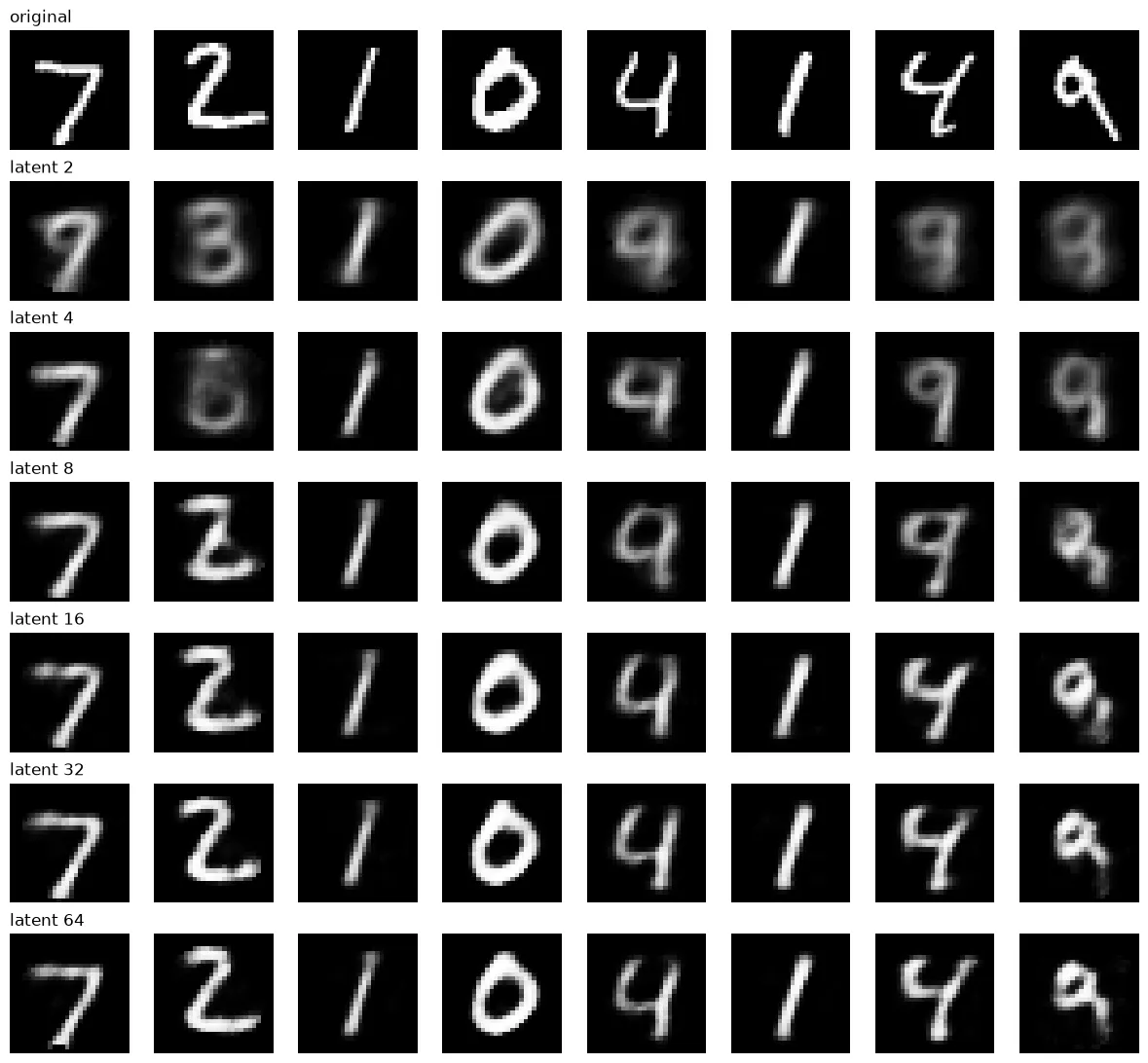
같은 테스트 이미지 8장을 잠재 차원별로 복원한 결과.
처음에는 숫자를 알아보려면 64차원 정도는 필요하지 않을까 예상했다. 하지만 그림에서는 2차원에서도 1이나 0처럼 읽을 수 있는 예시가 있고, 8~16차원에서는 더 많은 숫자의 형태가 드러난다. 차원을 더 늘리면 획과 필체도 원본에 가까워지는 모습이 보인다.
다만 두 질문은 나누어 봐야 한다.
- 어떤 숫자인지 사람이 알아볼 수 있는가?
- 원본의 획 두께, 기울기, 필체까지 보존하는가?
MSE는 픽셀 오차를 측정하므로 사람의 판독 가능성과 반드시 일치하지 않는다. 또한 차원을 늘리면 파라미터 수와 학습 양상도 달라진다. 한 번의 초기화와 5 epoch 결과만으로 특정 차원을 MNIST의 “실질적인 정보량”이라고 해석할 수는 없다.
4. 2차원 잠재 공간을 직접 들여다보기
잠재 차원이 2라면 이미지 하나를 평면의 점 하나로 표시할 수 있다. 테스트 이미지를 인코더에 넣어 z1, z2를 얻고, 해석을 위해 숫자 레이블로 색을 칠했다.
test_set = datasets.MNIST("./data", train=False, download=True,
                          transform=transforms.ToTensor())
test_loader = DataLoader(test_set, batch_size=1000)

model2 = results[2]["model"]
model2.eval()

zs, ys = [], []
with torch.no_grad():
    for images, labels in test_loader:
        x = torch.flatten(images, start_dim=1).to(device)
        zs.append(model2.encoder(x).cpu())
        ys.append(labels)

z = torch.cat(zs); y = torch.cat(ys)

plt.figure(figsize=(8, 7))
sc = plt.scatter(z[:, 0], z[:, 1], c=y, cmap="tab10", s=3, alpha=0.6)
plt.colorbar(sc, ticks=range(10))
plt.xlabel("z1"); plt.ylabel("z2")
plt.show()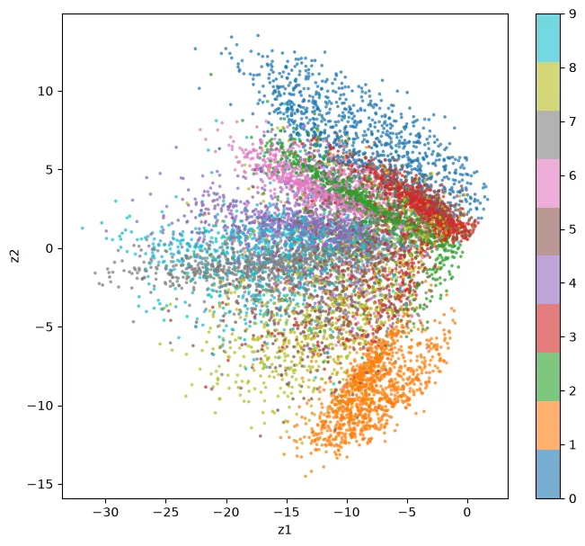
2차원 AE의 잠재 벡터. 색은 학습에 사용하지 않은 숫자 레이블이다.
같은 숫자의 이미지들이 일부 가까이 모이지만 서로 다른 숫자가 겹치는 영역도 있다. 복원을 위해 배운 형태적 특징이 숫자 구분과 연결되는 부분이 있다는 정도로 해석할 수 있다. 이 결과만으로 모델이 숫자의 의미를 이해했다고 단정하지는 않는다.
관측된 점이 없는 곳을 디코딩하면?
잠재 공간에서 한 숫자가 우세한 위치, 레이블이 섞인 위치, 관측점에서 떨어진 위치를 골라 디코더에 넣어보았다.
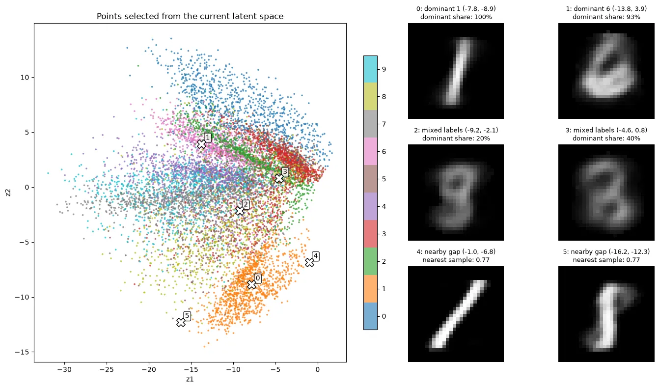
왼쪽의 X 좌표를 디코딩한 결과가 오른쪽에 표시되어 있다.
그림의 표시값은 다음과 같이 읽는다.
dominant share: 가까운 30개 점에서 가장 많은 숫자의 비율이다. 디코더의 분류 확률이 아니다.mixed labels: 주변 점들의 숫자 레이블이 섞인 후보 위치다.nearby gap: 관측된 테스트 잠재 벡터에서 떨어진 후보 위치다. 학습 데이터까지 전혀 없었던 곳이라는 뜻은 아니다.
원본 실습에서는 빈 공간 후보에서도 9와 1처럼 보이는 출력이 관찰되었다. 즉, “AE의 빈 공간에서는 숫자가 나오지 않는다”는 설명은 적절하지 않다.
남는 질문은 따로 있다. 새 이미지를 생성하려면 좌표를 어디서, 어떤 확률로 뽑아야 할까? 일반 AE의 복원 목표만으로는 그 분포가 정해지지 않는다. 이 질문은 뒤에서 VAE로 이어진다.
5. DAE: 손상된 입력에서 원본을 추정하기
이번에는 입력에 노이즈를 더해보자. 일반 AE와 DAE의 차이는 모델 구조보다 입력과 목표의 관계에 있다.
| 모델 | 학습 입력 | 복원 목표 |
|---|---|---|
| AE | 깨끗한 원본 x | 깨끗한 원본 x |
| DAE | 노이즈를 더한 입력 x̃ | 깨끗한 원본 x |
핵심 코드는 간단하다.
def add_noise(x, factor=0.3):
    return torch.clamp(x + factor * torch.randn_like(x), 0., 1.)

loss = criterion(dae(add_noise(x)), x)
입력에만 노이즈가 있고, 손실 함수의 목표는 여전히 깨끗한 원본이다. 모델은 손상된 입력을 그대로 복사하는 대신 원본을 추정해야 한다.
같은 노이즈 입력으로 AE와 DAE 비교하기
두 모델은 잠재 차원 16, 같은 초기 가중치, 같은 배치 순서, 같은 학습 횟수인 50 epoch를 사용했다. 평가 시에는 두 모델 모두 동일한 노이즈 테스트 이미지를 입력받았다.
| 평가 대상 | 원본 대비 테스트 MSE |
|---|---|
| 노이즈 입력 자체 | 0.0467 |
| 일반 AE의 출력 | 0.0514 |
| DAE의 출력 | 0.0146 |
세 값 모두 테스트 이미지 10,000장 전체의 픽셀당 평균 제곱 오차다.
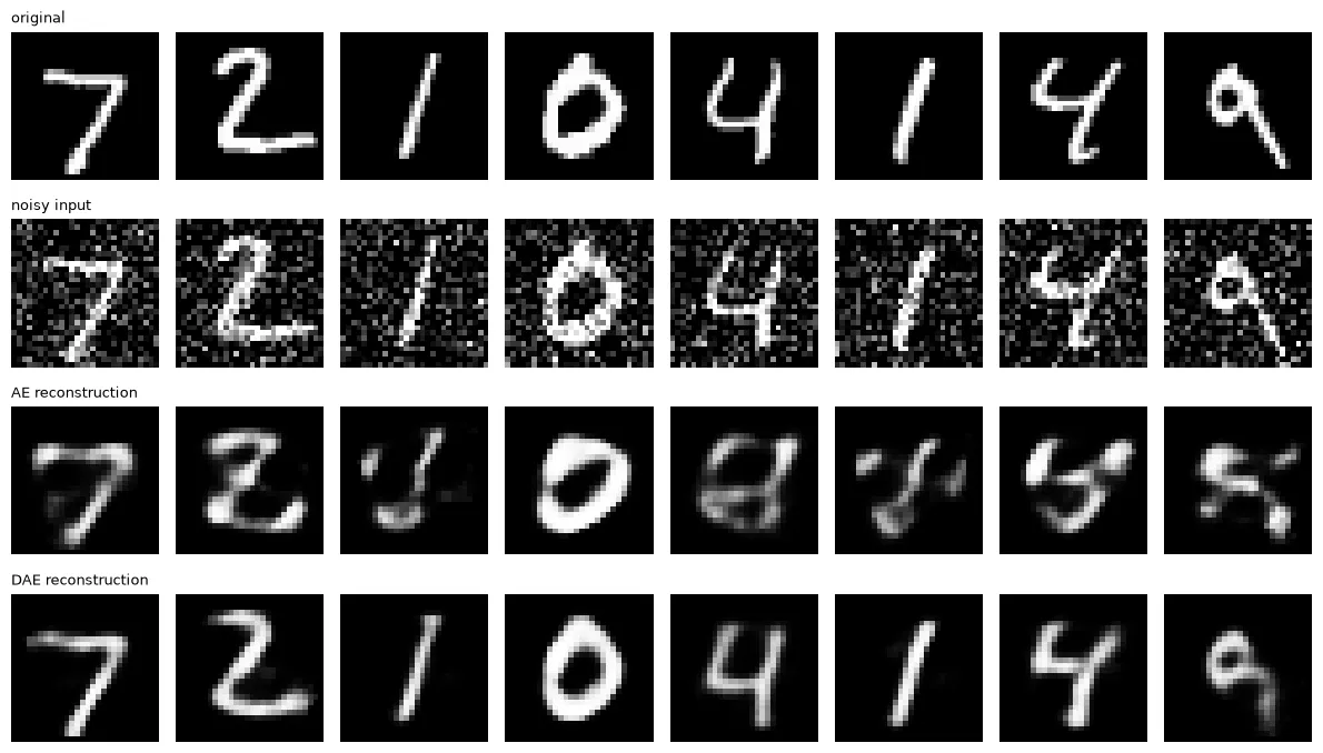
위에서부터 원본, 노이즈 입력, 일반 AE 출력, DAE 출력.
이번 결과에서 일반 AE는 노이즈 입력 자체보다 MSE가 높았다. 깨끗한 입력으로 복원을 학습했다고 해서 손상된 입력에서도 잘 복원하는 것은 아니라는 사례다.
반면 DAE는 노이즈를 줄이고 숫자 형태를 더 잘 복원했다. 다만 획과 필체까지 완벽하게 보존하지는 않았다. 노이즈를 얼마나 없앴는지와 원본의 특징을 얼마나 남겼는지를 함께 확인해야 한다.
이 비교는 현재 노이즈 종류와 세기에 대한 결과다. 모든 손상에 같은 성능을 보인다는 뜻은 아니다.
6. VAE: 새 좌표를 뽑을 분포까지 정하기
AE에서는 입력을 잠재 벡터 하나로 바꾸었다. 이번 VAE에서는 입력마다 잠재 벡터의 평균과 로그 분산을 계산한다.
입력 이미지 → 인코더 → mu, logvar → 잠재 벡터 z 샘플링 → 디코더 → 복원이미지별 잠재 분포를 이용해 원본을 복원하면서, 그 분포가 기준 분포인 표준정규분포에서 너무 멀어지지 않도록 학습한다.
분포는 숫자 클래스마다 하나씩 만들어지는 것이 아니라 입력 이미지마다 만들어진다. 생성할 때는 입력 이미지 없이 기준 분포에서 z를 뽑아 디코더에 넣는다.
Reparameterization trick
인코더가 출력한 logvar는 로그 분산이다. 이를 표준편차로 바꾼 뒤 표준정규분포 난수와 결합한다.
난수는 eps에서 뽑고, mu와 std에는 미분 가능한 연산을 적용한다. 이 경로를 통해 복원 손실의 기울기가 인코더까지 전달된다.
class VAE(nn.Module):
    def __init__(self, latent_dim=2):
        super().__init__()
        self.fc = nn.Sequential(nn.Linear(784, 128), nn.ReLU())
        # 이미지마다 잠재 좌표의 중심 mu를 계산
        # latent_dim=2라면 [mu1, mu2]처럼 숫자 2개를 출력
        self.fc_mu = nn.Linear(128, latent_dim)
        # 로그 연산을 하는 층이 아니라, 출력값을 로그 분산으로 사용하는 층
        # 아래 표준편차 계산과 KL 손실에서 이 의미로 사용함
        self.fc_logvar = nn.Linear(128, latent_dim)
        self.decoder = nn.Sequential(
            nn.Linear(latent_dim, 128), nn.ReLU(),
            nn.Linear(128, 784), nn.Sigmoid()
        )

    def encode(self, x):
        h = self.fc(x)
        return self.fc_mu(h), self.fc_logvar(h)

    def reparameterize(self, mu, logvar):
        # 로그 분산을 표준편차로 변환: std = exp(logvar / 2)
        std = torch.exp(0.5 * logvar)
        # 평균 0, 표준편차 1인 정규분포 난수
        # 각 좌표에서 중심으로부터 표준편차의 몇 배만큼 이동할지 정함
        eps = torch.randn_like(std)
        # 중심 + 이동량으로 잠재 좌표 계산
        return mu + eps * std

    def forward(self, x):
        mu, logvar = self.encode(x)
        z = self.reparameterize(mu, logvar)
        return self.decoder(z), mu, logvar
복원 손실과 KL 항
이번 실습의 손실은 복원 오차와 KL 항을 더한 것이다.
복원 항은 원본을 잘 되살리도록 하고, KL 항은 이미지별 분포의 평균과 분산이 기준 분포에 가까워지도록 작용한다.
# reconstruction: 원본과 복원 이미지의 픽셀별 제곱 오차 합
# KL: 이미지별 잠재 분포가 기준 분포에서 벗어난 정도
# 로그에서는 두 항과 합계를 각각 이미지 수로 나눕니다.
# reconstruction은 픽셀 평균 MSE가 아니라 이미지당 픽셀 오차 합입니다.
def vae_loss(recon, x, mu, logvar, return_components=False):
    recon_loss = F.mse_loss(recon, x, reduction="sum")
    kl = -0.5 * torch.sum(1 + logvar - mu.pow(2) - logvar.exp())
    total = recon_loss + kl
    if return_components:
        return total, recon_loss, kl
    return total
여기서 복원 항은 reduction="sum"을 사용한다. 로그를 출력할 때는 이미지 수로 나누므로, 앞에서 사용한 픽셀당 평균 MSE와 단위가 다르다. 복원 항과 KL 항의 합산 방식은 두 목표의 상대적인 크기에도 영향을 준다.
KL 항을 빼면 어떻게 될까? 모델은 복원 오차만 줄이면 되므로 표준편차를 작게 만들어 난수의 영향을 줄이는 방향으로 학습될 수 있다. 또한 이미지별 분포를 기준 분포에 맞출 이유가 사라져, 생성 시 표준정규분포에서 뽑은 좌표가 좋은 출력을 만든다고 기대하기 어려워진다.
그렇다고 KL 항이 모든 빈 공간을 채우거나 이미지를 반드시 선명하게 만드는 것은 아니다. 복원 목표와 분포 제약 사이에 절충이 생긴다.
2차원 VAE 학습하기
vae = VAE(latent_dim=2).to(device)
optimizer = torch.optim.Adam(vae.parameters(), lr=1e-3)

for epoch in range(20):
    vae.train()
    recon_total, kl_total, sample_count = 0.0, 0.0, 0
    for images, _ in train_loader:
        x = images.view(images.size(0), -1).to(device)
        recon, mu, logvar = vae(x)
        loss, recon_term, kl_term = vae_loss(
            recon, x, mu, logvar, return_components=True
        )
        optimizer.zero_grad(); loss.backward(); optimizer.step()
        recon_total += recon_term.item()
        kl_total += kl_term.item()
        sample_count += x.size(0)
    if (epoch+1) % 5 == 0:
        print(f"epoch {epoch+1} | per image: "
              f"reconstruction {recon_total/sample_count:.4f} | "
              f"KL {kl_total/sample_count:.4f} | "
f"total {(recon_total+kl_total)/sample_count:.4f}")| Epoch | 복원 항 / 이미지 | KL / 이미지 | 합계 / 이미지 |
|---|---|---|---|
| 5 | 39.5887 | 3.2838 | 42.8726 |
| 10 | 37.2238 | 3.6590 | 40.8828 |
| 15 | 36.0197 | 3.8960 | 39.9157 |
| 20 | 35.2477 | 4.0587 | 39.3064 |
학습 중 복원 항은 감소하고 KL 항은 증가했다. 합계는 감소했으므로 두 항을 함께 최적화하는 과정에서 나타난 변화로 읽을 수 있다. 각 항이 매번 동시에 감소해야 하는 것은 아니다.
7. 입력 이미지 없이 생성하기
학습이 끝나면 인코더를 거치지 않고 표준정규분포에서 잠재 벡터를 뽑는다.
# 입력 이미지와 인코더 없이, 기준 분포 N(0, I)에서 생성합니다.
vae.eval()
with torch.no_grad():
    z_new = torch.randn(16, vae.fc_mu.out_features, device=device)
    generated = vae.decoder(z_new).cpu().view(16, 28, 28)

fig, axes = plt.subplots(4, 4, figsize=(6, 6))
for i, ax in enumerate(axes.flat):
    ax.imshow(generated[i], cmap="gray", vmin=0, vmax=1)
    ax.axis("off")
fig.suptitle("VAE: samples from N(0, I)")
plt.tight_layout()
plt.show()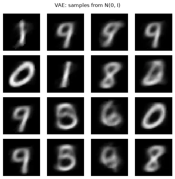
2차원 VAE의 기준 분포에서 잠재 벡터 16개를 뽑아 생성한 이미지.
이 결과는 주어진 원본의 복원이 아니다. 새로운 잠재 좌표를 디코더에 넣은 생성 결과다. 숫자 형태가 나타나지만 모든 결과가 선명하거나 명확한 것은 아니다.
잠재 차원을 16으로 늘리면?
같은 데이터, 배치 크기, 학습률, 손실 함수로 16차원 VAE를 별도로 20 epoch 학습했다.
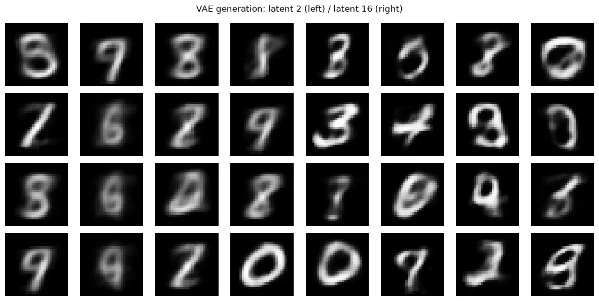
왼쪽: 잠재 차원 2 · 오른쪽: 잠재 차원 16. 각 모델의 잠재 공간은 서로 다르다.
이 예시에서는 오른쪽에 경계가 더 뚜렷한 숫자가 여러 개 보인다. 하지만 같은 칸에 같은 숫자가 나와야 하는 비교는 아니다. 두 모델의 잠재 좌표는 서로 대응하는 의미를 갖지 않는다.
20 epoch의 학습 로그도 비교하면 다음과 같다.
| 잠재 차원 | 복원 항 / 이미지 | KL / 이미지 | 합계 / 이미지 |
|---|---|---|---|
| 2 | 35.2477 | 4.0587 | 39.3064 |
| 16 | 20.1170 | 11.2927 | 31.4097 |
16차원 모델에서 복원 항은 작고 KL 항은 컸다. 차원이 늘면 파라미터 수와 KL을 합산하는 차원 수도 달라지고, 이번 두 모델의 초기화와 학습 순서도 같지 않다. 따라서 차원을 늘리면 반드시 생성 품질이 좋아진다는 결론 대신, 현재 설정에서의 탐색적 비교로 받아들이는 것이 적절하다.
잠재 좌표를 조금씩 이동해보기
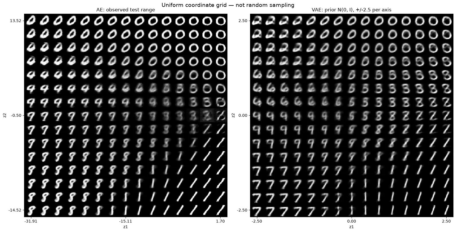
왼쪽: AE의 관측 잠재 범위 · 오른쪽: VAE의 각 축 -2.5~2.5 범위. 균일 간격의 좌표 격자다.
가로로 이동하면 z1, 세로로 이동하면 z2가 변한다. 이웃한 좌표에서 획과 숫자 형태가 어떻게 바뀌는지 볼 수 있다.
이 그림은 균일한 간격으로 좌표를 훑은 결과이며, 정규분포에서 무작위로 뽑은 결과가 아니다. AE와 VAE의 탐색 범위, 좌표 의미, 학습 횟수도 다르므로 이 그림 하나로 생성 성능의 우열을 판단하기는 어렵다.
8. 정리: 어떤 제약을 주느냐가 학습을 바꾼다
처음 질문은 “입력을 그대로 출력할 거라면 왜 학습할까?”였다. 실험을 따라가며 중요한 것은 어떤 경로로 복원하게 만드는지라는 점을 확인했다.
| 모델 | 이번 실습에서 준 제약 | 확인한 점 |
|---|---|---|
| AE | 좁은 잠재 공간을 거쳐 복원 | 차원에 따라 복원 오차와 보존되는 형태가 달라졌다. |
| DAE | 손상된 입력으로 깨끗한 원본 추정 | 해당 노이즈 조건에서 일반 AE보다 낮은 복원 오차를 보였다. |
| VAE | 이미지별 잠재 분포를 기준 분포에 가깝게 유도 | 기준 분포에서 좌표를 뽑아 입력 없이 이미지를 생성했다. |
이 과정에서 구분해야 할 것도 남았다.
- 낮은 복원 손실만으로 잠재 표현의 유용성을 판단할 수 없다.
- 노이즈 제거 성능과 원본의 세부 특징 보존은 함께 확인해야 한다.
- 몇 개의 그럴듯한 생성 이미지와 안정적인 생성 성능은 다르다.
이번 비교는 저장된 단일 실행 결과를 바탕으로 한다. 테스트 결과를 반복해서 보며 차원이나 학습 횟수를 선택하려면 별도의 검증 세트를 두어야 한다.
오토인코더의 흥미로운 점은 “복원”이라는 비슷한 목표에서도 병목, 손상된 입력, 확률분포라는 조건을 어떻게 주느냐에 따라 배우는 표현과 활용 방식이 달라진다는 것이다.
부록: 비교 실험과 시각화 코드
아래 코드는 본문에서 정의한 변수와 모델을 이어서 사용한다. DAE 학습과 16차원 VAE 학습은 환경에 따라 시간이 걸릴 수 있다.
AE 복원 그림
model.eval()
with torch.no_grad():
    images, _ = next(iter(train_loader))
    x = torch.flatten(images, start_dim=1).to(device)
    recon = model(x).cpu().view(-1, 28, 28)

fig, axes = plt.subplots(2, 8, figsize=(12, 3))
for i in range(8):
    # 원본
    axes[0, i].imshow(images[i].squeeze(), cmap="gray"); axes[0, i].axis("off")
    # 복원
    axes[1, i].imshow(recon[i], cmap="gray"); axes[1, i].axis("off")
plt.show()
잠재 차원별 복원 그림
# 섞지 않은 테스트 데이터의 첫 8장을 모든 모델에 똑같이 사용합니다.
images, _ = next(iter(test_loader))
images = images[:8]
x = torch.flatten(images, start_dim=1).to(device)

fig, axes = plt.subplots(len(latent_dims) + 1, 8, figsize=(12, 11))
for i in range(8):
    axes[0, i].imshow(images[i].squeeze(), cmap="gray", vmin=0, vmax=1)
    axes[0, i].axis("off")
axes[0, 0].set_title("original", loc="left")

for row, d in enumerate(latent_dims, start=1):
    model_d = results[d]["model"]
    model_d.eval()
    with torch.no_grad():
        recon = model_d(x).cpu().view(-1, 28, 28)
    for i in range(8):
        axes[row, i].imshow(recon[i], cmap="gray", vmin=0, vmax=1)
        axes[row, i].axis("off")
    axes[row, 0].set_title(f"latent {d}", loc="left")
plt.tight_layout()
plt.show()
AE 잠재 좌표 선택과 디코딩
model2 = results[2]["model"]
model2.eval()


def select_latent_points(z, y, neighbors=30):
    # CPU에서 현재 산점도의 이웃을 조사합니다. 레이블은 위치 해석에만 씁니다.
    coords = z.detach().cpu().float()
    labels = y.detach().cpu().long()
    k = min(neighbors, len(coords))
    candidates = coords[torch.linspace(0, len(coords) - 1,
                                       min(600, len(coords))).long()]
    distances, indices = torch.cdist(candidates, coords, compute_mode="donot_use_mm_for_euclid_dist").topk(k, largest=False)
    proportions = F.one_hot(labels[indices], num_classes=10).float().mean(1)
    purity, dominant = proportions.max(1)
    entropy = -(proportions * proportions.clamp_min(1e-12).log()).sum(1)
    radius = distances[:, -1]
    dense = radius <= torch.quantile(radius, 0.6)
    typical_radius = radius.median().clamp_min(1e-6)
    separation = (coords.max(0).values - coords.min(0).values).norm() * 0.12

    def pick_spaced(order, pool, count=2):
        chosen = []
        for index in order.tolist():
            if not chosen or torch.cdist(pool[index:index+1], pool[chosen]).min() >= separation:
                chosen.append(index)
            if len(chosen) == count:
                break
        # 분포가 좁아도 같은 후보를 중복 선택하지 않습니다.
        for index in order.tolist():
            if len(chosen) == count:
                break
            if index not in chosen:
                chosen.append(index)
        return chosen

    # 밀집한 후보에서 서로 다른 숫자가 우세한 위치를 고릅니다.
    dense_indices = torch.where(dense)[0]
    pure_order = dense_indices[torch.argsort(purity[dense_indices], descending=True)]
    first = pure_order[0].item()
    other_classes = pure_order[dominant[pure_order] != dominant[first]]
    second = other_classes[0].item() if len(other_classes) else pure_order[1].item()
    pure_indices = [first, second]

    # 밀집한 후보 중 주변 레이블이 많이 섞인 위치를 고릅니다.
    mixed_order = dense_indices[torch.argsort(entropy[dense_indices], descending=True)]
    mixed_order = mixed_order[(mixed_order != first) & (mixed_order != second)]
    high_entropy = mixed_order[entropy[mixed_order] >= 0.5 * entropy[mixed_order].max()]
    if len(high_entropy) >= 2:
        mixed_order = high_entropy
    mixed_indices = pick_spaced(mixed_order, candidates)

    # 관측 범위보다 조금 넓은 격자에서 실제 점과 적당히 떨어진 위치를 찾습니다.
    lower, upper = coords.min(0).values, coords.max(0).values
    padding = (upper - lower).clamp_min(1e-6) * 0.05
    gx = torch.linspace(lower[0] - padding[0], upper[0] + padding[0], 35)
    gy = torch.linspace(lower[1] - padding[1], upper[1] + padding[1], 35)
    xx, yy = torch.meshgrid(gx, gy, indexing="ij")
    grid = torch.stack([xx.flatten(), yy.flatten()], dim=1)
    nearest = torch.cat([
        torch.cdist(chunk, coords, compute_mode="donot_use_mm_for_euclid_dist").min(1).values
        for chunk in grid.split(128)
    ])
    # 가장 가까운 실제 점까지의 거리가 대표적인 이웃 반경의 1.5배에 가까운 후보를 고릅니다.
    gap_order = torch.argsort((nearest - 1.5 * typical_radius).abs())
    gap_indices = pick_spaced(gap_order, grid)

    points = torch.cat([candidates[pure_indices], candidates[mixed_indices], grid[gap_indices]])
    names = [f"dominant {dominant[j].item()}" for j in pure_indices]
    names += ["mixed labels" if entropy[j] > 0.1 else "low mixing" for j in mixed_indices]
    names += ["nearby gap", "nearby gap"]
    notes = [f"dominant share: {purity[j]:.0%}" for j in pure_indices + mixed_indices]
    notes += [f"nearest sample: {nearest[j]:.2f}" for j in gap_indices]
    return points, names, notes


points, point_names, point_notes = select_latent_points(z, y)
with torch.no_grad():
    images = model2.decoder(points.to(device)).cpu().view(-1, 28, 28).numpy()

fig = plt.figure(figsize=(14, 8))
gs = fig.add_gridspec(3, 4, width_ratios=[1, 1, 0.85, 0.85])
ax = fig.add_subplot(gs[:, :2])
sc = ax.scatter(z[:, 0], z[:, 1], c=y, cmap="tab10", s=3, alpha=0.6,
                vmin=-0.5, vmax=9.5)
fig.colorbar(sc, ax=ax, ticks=range(10), fraction=0.04)
for i, p in enumerate(points):
    ax.scatter(*p.tolist(), s=160, marker="X", c="white", edgecolors="black", zorder=5)
    ax.annotate(str(i), p.tolist(), xytext=(6, 6), textcoords="offset points",
                bbox=dict(boxstyle="round,pad=0.2", fc="white", alpha=0.8))
ax.set(xlabel="z1", ylabel="z2", title="Points selected from the current latent space")
for i in range(6):
    row, col = divmod(i, 2)
    im_ax = fig.add_subplot(gs[row, col + 2])
    im_ax.imshow(images[i], cmap="gray", vmin=0, vmax=1)
    px, py = points[i].tolist()
    im_ax.set_title(f"{i}: {point_names[i]} ({px:.1f}, {py:.1f})\n{point_notes[i]}", fontsize=9)
    im_ax.axis("off")
plt.tight_layout()
plt.show()
AE·DAE 동일 조건 학습과 평가
# 입력에만 노이즈를 더하고, 복원 목표는 원본으로 둡니다.
def add_noise(x, factor=0.3):
    return torch.clamp(x + factor * torch.randn_like(x), 0., 1.)


def evaluate_denoising(ae, dae, loader, factor, seed):
    ae.eval()
    dae.eval()
    # 평가할 때마다 같은 난수열로 각 이미지에 동일한 노이즈를 더합니다.
    noise_generator = torch.Generator().manual_seed(seed)
    totals = {"noisy input": 0.0, "AE": 0.0, "DAE": 0.0}
    pixels = 0
    with torch.no_grad():
        for images, _ in loader:
            clean_cpu = torch.flatten(images, start_dim=1)
            noise = torch.randn(clean_cpu.shape, generator=noise_generator)
            noisy = (clean_cpu + factor * noise).clamp(0, 1).to(device)
            clean = clean_cpu.to(device)
            outputs = {"noisy input": noisy, "AE": ae(noisy), "DAE": dae(noisy)}
            for name, output in outputs.items():
                totals[name] += F.mse_loss(output, clean, reduction="sum").item()
            pixels += clean.numel()
    return {name: total / pixels for name, total in totals.items()}


latent_dim = 16
epochs = 50
noise_factor = 0.3
torch.manual_seed(SEED)
ae_baseline = AutoEncoder(latent_dim=latent_dim).to(device)
dae = AutoEncoder(latent_dim=latent_dim).to(device)
# 동일한 초기 가중치에서 시작해 입력에 노이즈를 더하는 효과를 비교합니다.
dae.load_state_dict(ae_baseline.state_dict())
ae_optimizer = torch.optim.Adam(ae_baseline.parameters(), lr=1e-3)
dae_optimizer = torch.optim.Adam(dae.parameters(), lr=1e-3)
criterion = nn.MSELoss()
paired_loader = DataLoader(
    train_set, batch_size=256, shuffle=True,
    generator=torch.Generator().manual_seed(SEED)
)
test_loader_eval = DataLoader(test_set, batch_size=1000, shuffle=False)
train_hist, test_hist = [], []
ae_train_hist, ae_test_hist = [], []

for epoch in range(epochs):
    ae_baseline.train()
    dae.train()
    ae_total, dae_total, train_pixels = 0.0, 0.0, 0
    for images, _ in paired_loader:
        x = torch.flatten(images, start_dim=1).to(device)
        # 일반 AE: 원본 → 원본
        ae_loss = criterion(ae_baseline(x), x)
        ae_optimizer.zero_grad()
        ae_loss.backward()
        ae_optimizer.step()
        # DAE: 노이즈 입력 → 원본. 같은 미니배치로 같은 횟수만큼 업데이트합니다.
        dae_loss = criterion(dae(add_noise(x, noise_factor)), x)
        dae_optimizer.zero_grad()
        dae_loss.backward()
        dae_optimizer.step()
        ae_total += ae_loss.item() * x.numel()
        dae_total += dae_loss.item() * x.numel()
        train_pixels += x.numel()

    metrics = evaluate_denoising(ae_baseline, dae, test_loader_eval, noise_factor, SEED + 1)
    ae_train_hist.append(ae_total / train_pixels)
    train_hist.append(dae_total / train_pixels)
    ae_test_hist.append(metrics["AE"])
    test_hist.append(metrics["DAE"])
    if (epoch + 1) % 10 == 0 or epoch + 1 == epochs:
        print(f"epoch {epoch+1}: fixed noisy test MSE | "
              f"input {metrics['noisy input']:.4f} | "
              f"AE {metrics['AE']:.4f} | DAE {metrics['DAE']:.4f}")
# 평가와 동일한 테스트 이미지와 노이즈에서 첫 8장을 표시합니다.
images, _ = next(iter(test_loader_eval))
clean_cpu = torch.flatten(images, start_dim=1)
noise_generator = torch.Generator().manual_seed(SEED + 1)
noise = torch.randn(clean_cpu.shape, generator=noise_generator)
noisy_cpu = (clean_cpu + noise_factor * noise).clamp(0, 1)
x = clean_cpu[:8].to(device)
noisy = noisy_cpu[:8].to(device)
ae_baseline.eval()
dae.eval()
with torch.no_grad():
ae_out = ae_baseline(noisy).cpu().view(-1, 28, 28)
out = dae(noisy).cpu().view(-1, 28, 28)
rows = [images[:8].squeeze(1), noisy.cpu().view(-1, 28, 28), ae_out, out]
names = ["original", "noisy input", "AE reconstruction", "DAE reconstruction"]
fig, axes = plt.subplots(4, 8, figsize=(12, 7))
for row, (batch, name) in enumerate(zip(rows, names)):
for i in range(8):
axes[row, i].imshow(batch[i], cmap="gray", vmin=0, vmax=1)
axes[row, i].axis("off")
axes[row, 0].set_title(name, loc="left", fontsize=9)
plt.tight_layout()
plt.show()
# 표시한 8장만이 아니라 테스트 세트 전체의 평균 MSE입니다.
comparison_mse = evaluate_denoising(
ae_baseline, dae, test_loader_eval, noise_factor, SEED + 1
)
print(f"Test samples: {len(test_set)} | latent dim: {latent_dim} | epochs: {epochs}")
for name, mse in comparison_mse.items():
print(f"{name:>11}: MSE {mse:.4f}")16차원 VAE 학습과 생성 비교
# 기존 vae(2차원)는 유지하고 16차원 모델을 별도로 학습합니다.
torch.manual_seed(SEED)
vae16 = VAE(latent_dim=16).to(device)
optimizer16 = torch.optim.Adam(vae16.parameters(), lr=1e-3)
comparison_epochs = 20  # 위 2차원 VAE와 같은 학습 횟수
vae16_loader = DataLoader(
    train_set, batch_size=train_loader.batch_size, shuffle=True,
    generator=torch.Generator().manual_seed(SEED)
)

for epoch in range(comparison_epochs):
    vae16.train()
    recon_total16, kl_total16, sample_count16 = 0.0, 0.0, 0
    for images, _ in vae16_loader:
        x = torch.flatten(images, start_dim=1).to(device)
        recon, mu16, logvar16 = vae16(x)
        loss16, recon_term16, kl_term16 = vae_loss(
            recon, x, mu16, logvar16, return_components=True
        )
        optimizer16.zero_grad()
        loss16.backward()
        optimizer16.step()
        recon_total16 += recon_term16.item()
        kl_total16 += kl_term16.item()
        sample_count16 += x.size(0)
    if (epoch + 1) % 5 == 0 or epoch + 1 == comparison_epochs:
        print(f"latent 16 | epoch {epoch+1} | per image: "
              f"reconstruction {recon_total16/sample_count16:.4f} | "
              f"KL {kl_total16/sample_count16:.4f} | "
              f"total {(recon_total16+kl_total16)/sample_count16:.4f}")

# 고정된 난수로 생성 예시를 비교합니다. 각 모델의 z는 서로 다른 공간입니다.
sample_generator = torch.Generator().manual_seed(SEED + 2)
z16_compare = torch.randn(16, 16, generator=sample_generator)
z2_compare = z16_compare[:, :2]
vae.eval()
vae16.eval()
with torch.no_grad():
    samples2 = vae.decoder(z2_compare.to(device)).cpu().view(16, 28, 28)
    samples16 = vae16.decoder(z16_compare.to(device)).cpu().view(16, 28, 28)

fig, axes = plt.subplots(4, 8, figsize=(12, 6))
for i in range(16):
    row, col = divmod(i, 4)
    for offset, samples in [(0, samples2), (4, samples16)]:
        ax = axes[row, col + offset]
        ax.imshow(samples[i], cmap="gray", vmin=0, vmax=1)
        ax.axis("off")
fig.suptitle("VAE generation: latent 2 (left) / latent 16 (right)")
plt.tight_layout()
plt.show()
VAE의 평균 좌표와 숫자별 중심 디코딩
vae.eval()
zs, ys = [], []
with torch.no_grad():
    for imgs_b, labels in test_loader:

        xb = imgs_b.view(imgs_b.size(0), -1).to(device)
        mu, _ = vae.encode(xb)
        zs.append(mu.cpu()); ys.append(labels)
z_vae = torch.cat(zs); y_vae = torch.cat(ys)

print("std:", z_vae.std(dim=0).tolist())

# 1) 좌표를 먼저 정한다 — 숫자별 군집 중심
targets = [0, 1, 3, 7, 8, 9]
points, labels_txt = [], []
for d in targets:
    c = z_vae[y_vae == d].mean(dim=0)
    points.append([c[0].item(), c[1].item()])
    labels_txt.append(f"center of {d}")

# 2) 그 좌표로 이미지를 만든다
with torch.no_grad():
    pts = torch.tensor(points, dtype=torch.float32).to(device)
    gen = vae.decoder(pts).cpu().view(-1, 28, 28).numpy()

# 3) 그린다
fig = plt.figure(figsize=(13, 7))
ax = fig.add_axes([0.05, 0.08, 0.55, 0.85])

sc = ax.scatter(z_vae[:, 0], z_vae[:, 1], c=y_vae, cmap="tab10", s=3, alpha=0.6)
fig.colorbar(sc, ax=ax, ticks=range(10), fraction=0.04)

for i, p in enumerate(points):
    ax.scatter(p[0], p[1], s=200, marker="X",
               c="white", edgecolors="black", linewidths=1.5, zorder=5)
    ax.annotate(labels_txt[i], p, xytext=(6, 6), textcoords="offset points",
                fontsize=9, bbox=dict(boxstyle="round,pad=0.3", fc="white", alpha=0.8))

ax.set_xlabel("z1"); ax.set_ylabel("z2"); ax.set_title("VAE latent space")

for i in range(6):
    row, col = divmod(i, 2)
    im_ax = fig.add_axes([0.68 + col * 0.15, 0.68 - row * 0.28, 0.13, 0.22])
    im_ax.imshow(gen[i], cmap="gray")
    im_ax.set_title(f"{labels_txt[i]} ({points[i][0]:.1f},{points[i][1]:.1f})",
                    fontsize=8)
    im_ax.axis("off")

plt.show()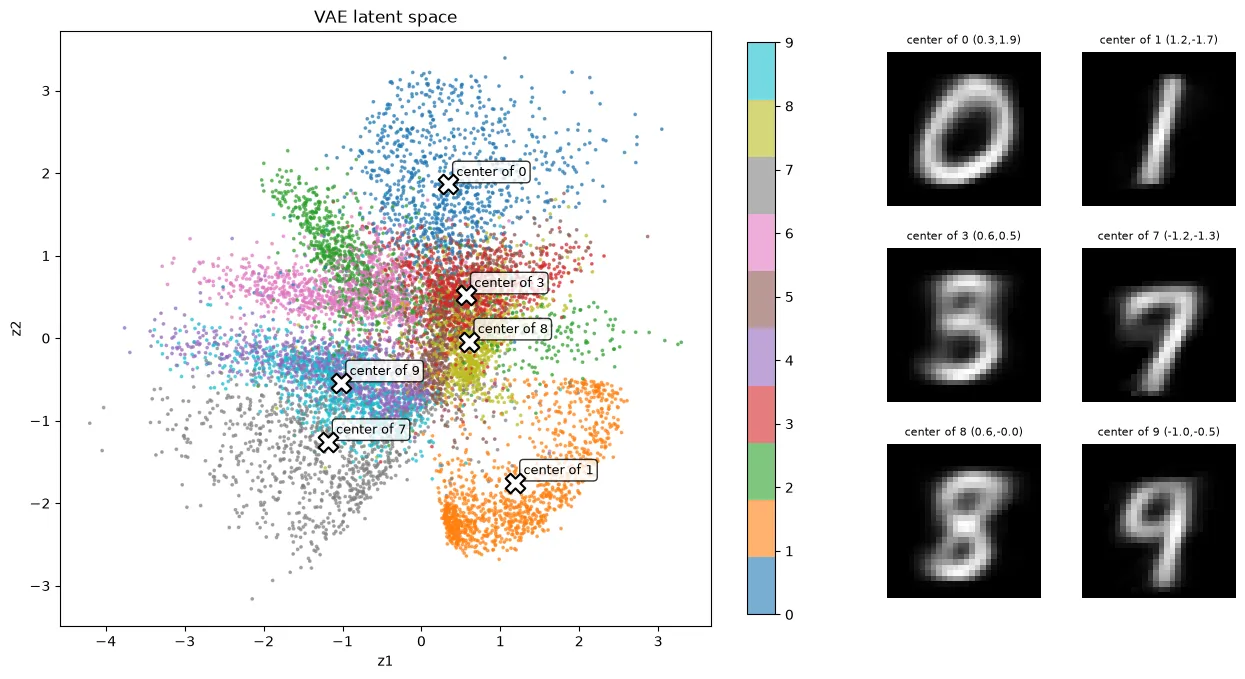
AE·VAE 잠재 격자 시각화
import numpy as np


def latent_grid(model_decoder, x_range, y_range, n=15, device=device):
    grid_x = np.linspace(*x_range, n)
    grid_y = np.linspace(*y_range, n)
    canvas = np.zeros((28*n, 28*n))
    with torch.no_grad():
        for i, yi in enumerate(grid_y[::-1]):
            pts = torch.tensor([[xj, yi] for xj in grid_x],
                               dtype=torch.float32, device=device)
            imgs = model_decoder(pts).cpu().view(-1, 28, 28).numpy()
            for j in range(n):
                canvas[i*28:(i+1)*28, j*28:(j+1)*28] = imgs[j]
    return canvas


ae2 = results[2]["model"]
ae2.eval()
vae.eval()
# 다른 셀의 z를 재사용하지 않고 현재 AE로 테스트 잠재 좌표를 계산합니다.
ae_grid_codes = []
with torch.no_grad():
    for images, _ in test_loader:
        x = torch.flatten(images, start_dim=1).to(device)
        ae_grid_codes.append(ae2.encoder(x).cpu())
ae_grid_codes = torch.cat(ae_grid_codes)
ae_lower = ae_grid_codes.min(dim=0).values
ae_upper = ae_grid_codes.max(dim=0).values
ae_x_range = (ae_lower[0].item(), ae_upper[0].item())
ae_y_range = (ae_lower[1].item(), ae_upper[1].item())

# VAE는 관측된 mu 범위가 아니라 기준 분포 N(0,I)의 중심 주변을 탐색합니다.
vae_x_range = (-2.5, 2.5)
vae_y_range = (-2.5, 2.5)
grid_n = 15
ae_canvas = latent_grid(ae2.decoder, ae_x_range, ae_y_range, n=grid_n)
vae_canvas = latent_grid(vae.decoder, vae_x_range, vae_y_range, n=grid_n)

fig, axes = plt.subplots(1, 2, figsize=(16, 8))
panels = [
    (ae_canvas, "AE: observed test range", ae_x_range, ae_y_range),
    (vae_canvas, "VAE: prior N(0, I), +/-2.5 per axis", vae_x_range, vae_y_range),
]
tick_indices = np.array([0, grid_n // 2, grid_n - 1])
# 각 타일의 중심에 실제 디코딩한 좌표를 표시합니다.
tick_positions = tick_indices * 28 + 13.5
for ax, (canvas, title, x_range, y_range) in zip(axes, panels):
    ax.imshow(canvas, cmap="gray", vmin=0, vmax=1, interpolation="nearest")
    ax.set_xticks(tick_positions, [f"{v:.2f}" for v in np.linspace(*x_range, grid_n)[tick_indices]])
    ax.set_yticks(tick_positions, [f"{v:.2f}" for v in np.linspace(*y_range, grid_n)[::-1][tick_indices]])
    ax.set_xlabel("z1")
    ax.set_ylabel("z2")
    ax.set_title(title, fontsize=12)
fig.suptitle("Uniform coordinate grid — not random sampling", fontsize=14)
plt.tight_layout()
plt.show()
When you first meet autoencoders, even the goal feels strange. Training a model to output exactly the image it was given — wouldn’t a single line of return x do the job?
But the story changes if the input has to pass through a narrow passage. To represent 784 pixels with fewer values and then restore them, the model has to learn which features to keep.
In this post we look at three models using MNIST handwritten digits.
| Model | How it learns | Question to explore |
|---|---|---|
| AE · Autoencoder | Compress the input, then restore it | What survives in a small latent vector? |
| DAE · Denoising Autoencoder | Restore the original from a corrupted input | What does it learn when we add noise? |
| VAE · Variational Autoencoder | Restore via a per-image latent distribution, pulled toward a reference distribution | Where do we sample coordinates to make new images? |
The numbers and figures below are execution results saved in the practice notebook. Re-running may give different results depending on model initialization, random numbers and the environment. The main text has the key code; the longer comparison and visualization code is collected in the appendix at the end.
1. Setup: a 28×28 image as a 784-dimensional vector
MNIST images are 28×28 grayscale images. ToTensor() turns the pixels into a tensor in the 0–1 range, and they are flattened to 784 dimensions before going into fully connected layers.
Install the required packages as follows.
pip install torch torchvision matplotlibBelow is the environment setup from the original notebook. It uses MPS on Apple Silicon if available, and otherwise runs on the CPU.
import torch
import torch.nn as nn
import torch.nn.functional as F
from torch.utils.data import DataLoader
from torchvision import datasets, transforms
import matplotlib.pyplot as plt

# 모델 초기화와 노이즈 생성 등에 사용할 공통 시드입니다.
SEED = 42
torch.manual_seed(SEED)

device = "mps" if torch.backends.mps.is_available() else "cpu"

train_set = datasets.MNIST("./data", train=True, download=True,
                           transform=transforms.ToTensor())
train_loader = DataLoader(train_set, batch_size=256, shuffle=True)
The DataLoader serves the training data in batches of 256 images. This is a choice to control how much is processed at once and how many updates happen.
torch.flatten(images, start_dim=1) merges only the image dimensions while keeping the batch dimension.
[배치 크기, 1, 28, 28] → [배치 크기, 784]2. AE: a bottleneck that forces it to learn reconstruction
An AE consists of an encoder and a decoder.
- Encoder: turns the input
xinto a latent vectorz. - Decoder: builds the reconstructed image
x̂from the latent vectorz.
The model’s structure is as follows.
입력 784 → 은닉층 128 → 잠재 벡터 32 → 은닉층 128 → 출력 784The latent vector is a summary representation used to restore the image. The bottleneck makes it hard to pass information through unchanged, but it does not automatically guarantee the semantic features a person would want.
class AutoEncoder(nn.Module):
    #잠재표현 층을 몇 차원으로 줄건지 latent_dim으로 받음.
    def __init__(self, latent_dim):
        super().__init__()
        #encoder
        self.encoder = nn.Sequential(
            nn.Linear(784, 128),
            nn.ReLU(),
            nn.Linear(128, latent_dim)
        )
        #decoder
        self.decoder = nn.Sequential(
            nn.Linear(latent_dim, 128),
            nn.ReLU(),
            nn.Linear(128, 784),
            nn.Sigmoid()
        )
    #forward = 순전파
    def forward(self, x):
        z = self.encoder(x)
        return self.decoder(z)
The final Sigmoid limits output pixels to the 0–1 range. In forward(), the input is encoded and then immediately decoded.
Using the input itself as the target instead of digit labels
The digit class labels are not used during training. Instead, it minimizes the MSE — the mean squared error per pixel — between the reconstruction and the input image.
Here, “not using labels” does not mean “there is no learning target”. The input image itself is the reconstruction target. MSE is the reconstruction loss chosen for this exercise; the fact that pixels are continuous does not mean MSE is the only option.
model = AutoEncoder(latent_dim=32).to(device)
criterion = nn.MSELoss()
optimizer = torch.optim.Adam(model.parameters(), lr=1e-3)

for epoch in range(5):
    total = 0
    for images, _ in train_loader:
        #start_dim=1: 1번 차원부터 합치기를 시작합니다. (보통 0번 차원은 배치 크기(Batch Size)이므로 유지합니다.)
        x = torch.flatten(images, start_dim=1).to(device)

        output = model(x)
        loss = criterion(output, x)

        optimizer.zero_grad()
        loss.backward()
        optimizer.step()

        total += loss.item()
    print(f"epoch {epoch+1}: {total/len(train_loader):.4f}")
The saved training log is below. These values are a training metric: the average of each epoch’s per-batch mean losses.
epoch 1: 0.0645
epoch 2: 0.0304
epoch 3: 0.0210
epoch 4: 0.0172
epoch 5: 0.0151
The loss went down. Let’s check the actual reconstructions too.
Top: original images · Bottom: reconstructions from an AE with latent dimension 32. Examples drawn from the training data.
If we raise the latent dimension to 784, does it copy perfectly?
In the current model, raising only the latent dimension gives this structure.
784 → 128 → 784 → 128 → 784There is still a 128-dimensional layer. So you cannot say the bottleneck is gone just because the latent dimension equals the input’s.
If the intermediate layers are widened too and the structure and activation functions allow it, the network can represent the identity function, but whether training actually reaches that solution is a separate matter. You also need to distinguish an identity function that returns even unseen inputs unchanged from overfitting that just memorizes the training data.
The key point is that reconstructing well and learning representations that are useful for other tasks are different things to evaluate.
3. What do we lose when we shrink the latent dimension?
I compared latent dimensions of 2, 4, 8, 16, 32, 64. Every model was trained for 5 epochs on training batches in the same order. Evaluation used the per-pixel mean MSE over all 10,000 test images.
# 모든 잠재 차원을 동일한 테스트 데이터로 평가합니다.
test_set = datasets.MNIST("./data", train=False, download=True,
                          transform=transforms.ToTensor())
test_loader = DataLoader(test_set, batch_size=1000, shuffle=False)
latent_dims = [2, 4, 8, 16, 32, 64]


def evaluate_mse(model, loader):
    model.eval()
    squared_error = 0.0
    pixel_count = 0
    with torch.no_grad():
        for images, _ in loader:
            x = torch.flatten(images, start_dim=1).to(device)
            recon = model(x)
            squared_error += F.mse_loss(
                recon, x, reduction="sum"
            ).item()
            pixel_count += x.numel()
    return squared_error / pixel_count


results = {}

for d in latent_dims:
    model = AutoEncoder(latent_dim=d).to(device)
    criterion = nn.MSELoss()
    optimizer = torch.optim.Adam(model.parameters(), lr=1e-3)
    # 모델 크기별 초기화 난수 소비량과 무관하게 같은 배치 순서를 사용합니다.
    comparison_loader = DataLoader(
        train_set, batch_size=256, shuffle=True,
        generator=torch.Generator().manual_seed(SEED)
    )

    for epoch in range(5):
        model.train()
        for images, _ in comparison_loader:
            x = torch.flatten(images, start_dim=1).to(device)
            loss = criterion(model(x), x)
            optimizer.zero_grad()
            loss.backward()
            optimizer.step()

    test_mse = evaluate_mse(model, test_loader)
    results[d] = {"model": model, "test_mse": test_mse}
print(f"latent {d:>2}: test MSE {test_mse:.4f}")| Latent dimension | Test MSE |
|---|---|
| 2 | 0.0488 |
| 4 | 0.0357 |
| 8 | 0.0249 |
| 16 | 0.0188 |
| 32 | 0.0135 |
| 64 | 0.0125 |
In this run, test MSE decreased as the dimension grew. Going from 32 to 64 still improved it, but only by 0.0010.
The same 8 test images reconstructed at each latent dimension.
At first I expected that recognizing the digits would need something like 64 dimensions. But in the figure, some examples are readable as a 1 or a 0 even at 2 dimensions, and at 8–16 dimensions the shapes of more digits emerge. With more dimensions, the strokes and handwriting also get closer to the original.
Two questions should be kept apart, though.
- Can a person tell which digit it is?
- Does it preserve the original’s stroke thickness, slant and handwriting?
MSE measures pixel error, so it does not necessarily match human readability. Increasing the dimension also changes the number of parameters and how training behaves. From a single initialization and 5 epochs, you cannot interpret any particular dimension as MNIST’s “effective amount of information”.
4. Looking directly into a 2D latent space
With a latent dimension of 2, each image can be shown as a single point on a plane. I fed the test images to the encoder to get z1 and z2, and colored them by digit label for interpretation.
test_set = datasets.MNIST("./data", train=False, download=True,
                          transform=transforms.ToTensor())
test_loader = DataLoader(test_set, batch_size=1000)

model2 = results[2]["model"]
model2.eval()

zs, ys = [], []
with torch.no_grad():
    for images, labels in test_loader:
        x = torch.flatten(images, start_dim=1).to(device)
        zs.append(model2.encoder(x).cpu())
        ys.append(labels)

z = torch.cat(zs); y = torch.cat(ys)

plt.figure(figsize=(8, 7))
sc = plt.scatter(z[:, 0], z[:, 1], c=y, cmap="tab10", s=3, alpha=0.6)
plt.colorbar(sc, ticks=range(10))
plt.xlabel("z1"); plt.ylabel("z2")
plt.show()
Latent vectors of the 2D AE. Colors are digit labels that were not used in training.
Images of the same digit partly cluster together, but there are also regions where different digits overlap. The most you can say is that the shape features learned for reconstruction are partly connected to telling digits apart. This result alone does not show that the model understands what the digits mean.
What if we decode a place with no observed points?
I picked locations in the latent space where one digit dominates, where labels are mixed, and away from the observed points, and fed them to the decoder.
The X coordinates on the left are decoded into the results shown on the right.
Read the labels in the figure as follows.
dominant share: the share of the most common digit among the 30 nearest points. It is not a classification probability from the decoder.mixed labels: candidate locations where the digit labels of nearby points are mixed.nearby gap: candidate locations away from the observed test latent vectors. It does not mean there was no training data there at all.
In the original notebook, outputs that looked like a 9 and a 1 appeared even at the empty-space candidates. So the explanation that “no digits come out of the empty space of an AE” is not accurate.
The remaining question is a different one: to generate new images, where, and with what probability, should we sample coordinates? The reconstruction objective of a plain AE does not define that distribution. This question leads to the VAE later on.
5. DAE: estimating the original from a corrupted input
Now let’s add noise to the input. The difference between a plain AE and a DAE lies less in the model architecture than in the relationship between the input and the target.
| Model | Training input | Reconstruction target |
|---|---|---|
| AE | Clean original x | Clean original x |
| DAE | Noisy input x̃ | Clean original x |
The key code is simple.
def add_noise(x, factor=0.3):
    return torch.clamp(x + factor * torch.randn_like(x), 0., 1.)

loss = criterion(dae(add_noise(x)), x)
Only the input has noise; the target of the loss is still the clean original. Instead of copying the corrupted input, the model has to estimate the original.
Comparing AE and DAE on the same noisy input
Both models used latent dimension 16, the same initial weights, the same batch order and the same 50 epochs of training. At evaluation, both received the same noisy test images.
| Evaluated | Test MSE against the original |
|---|---|
| The noisy input itself | 0.0467 |
| Plain AE output | 0.0514 |
| DAE output | 0.0146 |
All three values are the per-pixel mean squared error over all 10,000 test images.
From the top: original, noisy input, plain AE output, DAE output.
In this result, the plain AE had a higher MSE than the noisy input itself. It is an example showing that learning to reconstruct from clean inputs does not mean reconstructing well from corrupted ones.
The DAE, on the other hand, reduced the noise and restored the digit shapes better. It did not perfectly preserve the strokes and handwriting, though. You need to check both how much noise was removed and how much of the original’s character was kept.
This comparison is for the current noise type and strength. It does not mean the same performance holds for every kind of corruption.
6. VAE: defining the distribution for sampling new coordinates
In the AE, each input became a single latent vector. In this VAE, the mean and log-variance of the latent vector are computed for each input.
입력 이미지 → 인코더 → mu, logvar → 잠재 벡터 z 샘플링 → 디코더 → 복원It learns to reconstruct the original using a per-image latent distribution, while keeping that distribution from drifting too far from the reference distribution, a standard normal.
A distribution is created for each input image, not one per digit class. When generating, z is drawn from the reference distribution with no input image and fed to the decoder.
Reparameterization trick
The logvar output by the encoder is the log-variance. It is converted to a standard deviation and combined with standard normal noise.
The randomness is drawn in eps, and differentiable operations are applied to mu and std. Through this path, the gradient of the reconstruction loss reaches the encoder.
class VAE(nn.Module):
    def __init__(self, latent_dim=2):
        super().__init__()
        self.fc = nn.Sequential(nn.Linear(784, 128), nn.ReLU())
        # 이미지마다 잠재 좌표의 중심 mu를 계산
        # latent_dim=2라면 [mu1, mu2]처럼 숫자 2개를 출력
        self.fc_mu = nn.Linear(128, latent_dim)
        # 로그 연산을 하는 층이 아니라, 출력값을 로그 분산으로 사용하는 층
        # 아래 표준편차 계산과 KL 손실에서 이 의미로 사용함
        self.fc_logvar = nn.Linear(128, latent_dim)
        self.decoder = nn.Sequential(
            nn.Linear(latent_dim, 128), nn.ReLU(),
            nn.Linear(128, 784), nn.Sigmoid()
        )

    def encode(self, x):
        h = self.fc(x)
        return self.fc_mu(h), self.fc_logvar(h)

    def reparameterize(self, mu, logvar):
        # 로그 분산을 표준편차로 변환: std = exp(logvar / 2)
        std = torch.exp(0.5 * logvar)
        # 평균 0, 표준편차 1인 정규분포 난수
        # 각 좌표에서 중심으로부터 표준편차의 몇 배만큼 이동할지 정함
        eps = torch.randn_like(std)
        # 중심 + 이동량으로 잠재 좌표 계산
        return mu + eps * std

    def forward(self, x):
        mu, logvar = self.encode(x)
        z = self.reparameterize(mu, logvar)
        return self.decoder(z), mu, logvar
Reconstruction loss and the KL term
The loss in this exercise is the reconstruction error plus the KL term.
The reconstruction term pushes it to restore the original well, and the KL term pulls the mean and variance of each image’s distribution toward the reference distribution.
# reconstruction: 원본과 복원 이미지의 픽셀별 제곱 오차 합
# KL: 이미지별 잠재 분포가 기준 분포에서 벗어난 정도
# 로그에서는 두 항과 합계를 각각 이미지 수로 나눕니다.
# reconstruction은 픽셀 평균 MSE가 아니라 이미지당 픽셀 오차 합입니다.
def vae_loss(recon, x, mu, logvar, return_components=False):
    recon_loss = F.mse_loss(recon, x, reduction="sum")
    kl = -0.5 * torch.sum(1 + logvar - mu.pow(2) - logvar.exp())
    total = recon_loss + kl
    if return_components:
        return total, recon_loss, kl
    return total
Here the reconstruction term uses reduction="sum". When logging, it is divided by the number of images, so its units differ from the per-pixel mean MSE used earlier. How the reconstruction and KL terms are summed also affects the relative size of the two objectives.
What happens if we remove the KL term? The model only has to reduce reconstruction error, so it may learn to make the standard deviation small and reduce the effect of the noise. There is also no reason left to fit each image’s distribution to the reference distribution, so it becomes hard to expect coordinates drawn from a standard normal to produce good outputs at generation time.
That does not mean the KL term fills every empty space or always makes images sharp. A compromise forms between the reconstruction objective and the distribution constraint.
Training a 2D VAE
vae = VAE(latent_dim=2).to(device)
optimizer = torch.optim.Adam(vae.parameters(), lr=1e-3)

for epoch in range(20):
    vae.train()
    recon_total, kl_total, sample_count = 0.0, 0.0, 0
    for images, _ in train_loader:
        x = images.view(images.size(0), -1).to(device)
        recon, mu, logvar = vae(x)
        loss, recon_term, kl_term = vae_loss(
            recon, x, mu, logvar, return_components=True
        )
        optimizer.zero_grad(); loss.backward(); optimizer.step()
        recon_total += recon_term.item()
        kl_total += kl_term.item()
        sample_count += x.size(0)
    if (epoch+1) % 5 == 0:
        print(f"epoch {epoch+1} | per image: "
              f"reconstruction {recon_total/sample_count:.4f} | "
              f"KL {kl_total/sample_count:.4f} | "
f"total {(recon_total+kl_total)/sample_count:.4f}")| Epoch | Reconstruction / image | KL / image | Total / image |
|---|---|---|---|
| 5 | 39.5887 | 3.2838 | 42.8726 |
| 10 | 37.2238 | 3.6590 | 40.8828 |
| 15 | 36.0197 | 3.8960 | 39.9157 |
| 20 | 35.2477 | 4.0587 | 39.3064 |
During training the reconstruction term decreased and the KL term increased. The total decreased, so this can be read as a change that appears while optimizing the two terms together. Each term does not have to decrease at the same time every step.
7. Generating without an input image
Once training is done, latent vectors are drawn from the standard normal without going through the encoder.
# 입력 이미지와 인코더 없이, 기준 분포 N(0, I)에서 생성합니다.
vae.eval()
with torch.no_grad():
    z_new = torch.randn(16, vae.fc_mu.out_features, device=device)
    generated = vae.decoder(z_new).cpu().view(16, 28, 28)

fig, axes = plt.subplots(4, 4, figsize=(6, 6))
for i, ax in enumerate(axes.flat):
    ax.imshow(generated[i], cmap="gray", vmin=0, vmax=1)
    ax.axis("off")
fig.suptitle("VAE: samples from N(0, I)")
plt.tight_layout()
plt.show()
Images generated from 16 latent vectors drawn from the reference distribution of the 2D VAE.
These are not reconstructions of given originals. They are generated by feeding new latent coordinates to the decoder. Digit shapes appear, but not every result is sharp or clear.
What if we raise the latent dimension to 16?
With the same data, batch size, learning rate and loss function, I separately trained a 16-dimensional VAE for 20 epochs.
Left: latent dimension 2 · Right: latent dimension 16. Each model’s latent space is different.
In this example, several digits on the right have sharper edges. But this is not a comparison where the same cell should show the same digit. The two models’ latent coordinates do not correspond in meaning.
Comparing the 20-epoch training logs:
| Latent dimension | Reconstruction / image | KL / image | Total / image |
|---|---|---|---|
| 2 | 35.2477 | 4.0587 | 39.3064 |
| 16 | 20.1170 | 11.2927 | 31.4097 |
The 16-dimensional model had a smaller reconstruction term and a larger KL term. Increasing the dimension changes the number of parameters and the number of dimensions summed in the KL, and these two models also differed in initialization and training order. So rather than concluding that more dimensions always improve generation quality, it is better to take this as an exploratory comparison under the current settings.
Moving the latent coordinates little by little
Left: the AE’s observed latent range · Right: the VAE’s -2.5 to 2.5 range on each axis. Evenly spaced coordinate grids.
Moving horizontally changes z1, and moving vertically changes z2. You can see how strokes and digit shapes change between neighboring coordinates.
This figure is the result of sweeping coordinates at even intervals, not random draws from a normal distribution. The AE and VAE also differ in search range, coordinate meaning and training length, so this one figure is not enough to judge which generates better.
8. Summary: the constraint you impose changes what is learned
The original question was “why train it if it is just going to output the input?” Following the experiments, we saw that what matters is the path through which you make it reconstruct.
| Model | Constraint in this exercise | What we found |
|---|---|---|
| AE | Reconstruct through a narrow latent space | Reconstruction error and preserved shape changed with the dimension. |
| DAE | Estimate the clean original from a corrupted input | Showed lower reconstruction error than a plain AE under this noise condition. |
| VAE | Pull per-image latent distributions toward a reference distribution | Generated images without input by sampling coordinates from the reference distribution. |
Some distinctions also remain.
- Low reconstruction loss alone cannot tell you how useful a latent representation is.
- Denoising performance and preservation of the original’s fine details need to be checked together.
- A few plausible generated images are not the same as stable generation performance.
This comparison is based on a single saved run. If you want to choose the dimension or training length while repeatedly looking at results, you need a separate validation set.
What makes autoencoders interesting is that even with a similar goal of “reconstruction”, the representations they learn and how they can be used change depending on the conditions you set: a bottleneck, corrupted inputs, or a probability distribution.
Appendix: comparison experiments and visualization code
The code below continues to use the variables and models defined in the main text. DAE training and 16-dimensional VAE training may take a while depending on your environment.
AE reconstruction figure
model.eval()
with torch.no_grad():
    images, _ = next(iter(train_loader))
    x = torch.flatten(images, start_dim=1).to(device)
    recon = model(x).cpu().view(-1, 28, 28)

fig, axes = plt.subplots(2, 8, figsize=(12, 3))
for i in range(8):
    # 원본
    axes[0, i].imshow(images[i].squeeze(), cmap="gray"); axes[0, i].axis("off")
    # 복원
    axes[1, i].imshow(recon[i], cmap="gray"); axes[1, i].axis("off")
plt.show()
Reconstruction figure by latent dimension
# 섞지 않은 테스트 데이터의 첫 8장을 모든 모델에 똑같이 사용합니다.
images, _ = next(iter(test_loader))
images = images[:8]
x = torch.flatten(images, start_dim=1).to(device)

fig, axes = plt.subplots(len(latent_dims) + 1, 8, figsize=(12, 11))
for i in range(8):
    axes[0, i].imshow(images[i].squeeze(), cmap="gray", vmin=0, vmax=1)
    axes[0, i].axis("off")
axes[0, 0].set_title("original", loc="left")

for row, d in enumerate(latent_dims, start=1):
    model_d = results[d]["model"]
    model_d.eval()
    with torch.no_grad():
        recon = model_d(x).cpu().view(-1, 28, 28)
    for i in range(8):
        axes[row, i].imshow(recon[i], cmap="gray", vmin=0, vmax=1)
        axes[row, i].axis("off")
    axes[row, 0].set_title(f"latent {d}", loc="left")
plt.tight_layout()
plt.show()
Choosing and decoding AE latent coordinates
model2 = results[2]["model"]
model2.eval()


def select_latent_points(z, y, neighbors=30):
    # CPU에서 현재 산점도의 이웃을 조사합니다. 레이블은 위치 해석에만 씁니다.
    coords = z.detach().cpu().float()
    labels = y.detach().cpu().long()
    k = min(neighbors, len(coords))
    candidates = coords[torch.linspace(0, len(coords) - 1,
                                       min(600, len(coords))).long()]
    distances, indices = torch.cdist(candidates, coords, compute_mode="donot_use_mm_for_euclid_dist").topk(k, largest=False)
    proportions = F.one_hot(labels[indices], num_classes=10).float().mean(1)
    purity, dominant = proportions.max(1)
    entropy = -(proportions * proportions.clamp_min(1e-12).log()).sum(1)
    radius = distances[:, -1]
    dense = radius <= torch.quantile(radius, 0.6)
    typical_radius = radius.median().clamp_min(1e-6)
    separation = (coords.max(0).values - coords.min(0).values).norm() * 0.12

    def pick_spaced(order, pool, count=2):
        chosen = []
        for index in order.tolist():
            if not chosen or torch.cdist(pool[index:index+1], pool[chosen]).min() >= separation:
                chosen.append(index)
            if len(chosen) == count:
                break
        # 분포가 좁아도 같은 후보를 중복 선택하지 않습니다.
        for index in order.tolist():
            if len(chosen) == count:
                break
            if index not in chosen:
                chosen.append(index)
        return chosen

    # 밀집한 후보에서 서로 다른 숫자가 우세한 위치를 고릅니다.
    dense_indices = torch.where(dense)[0]
    pure_order = dense_indices[torch.argsort(purity[dense_indices], descending=True)]
    first = pure_order[0].item()
    other_classes = pure_order[dominant[pure_order] != dominant[first]]
    second = other_classes[0].item() if len(other_classes) else pure_order[1].item()
    pure_indices = [first, second]

    # 밀집한 후보 중 주변 레이블이 많이 섞인 위치를 고릅니다.
    mixed_order = dense_indices[torch.argsort(entropy[dense_indices], descending=True)]
    mixed_order = mixed_order[(mixed_order != first) & (mixed_order != second)]
    high_entropy = mixed_order[entropy[mixed_order] >= 0.5 * entropy[mixed_order].max()]
    if len(high_entropy) >= 2:
        mixed_order = high_entropy
    mixed_indices = pick_spaced(mixed_order, candidates)

    # 관측 범위보다 조금 넓은 격자에서 실제 점과 적당히 떨어진 위치를 찾습니다.
    lower, upper = coords.min(0).values, coords.max(0).values
    padding = (upper - lower).clamp_min(1e-6) * 0.05
    gx = torch.linspace(lower[0] - padding[0], upper[0] + padding[0], 35)
    gy = torch.linspace(lower[1] - padding[1], upper[1] + padding[1], 35)
    xx, yy = torch.meshgrid(gx, gy, indexing="ij")
    grid = torch.stack([xx.flatten(), yy.flatten()], dim=1)
    nearest = torch.cat([
        torch.cdist(chunk, coords, compute_mode="donot_use_mm_for_euclid_dist").min(1).values
        for chunk in grid.split(128)
    ])
    # 가장 가까운 실제 점까지의 거리가 대표적인 이웃 반경의 1.5배에 가까운 후보를 고릅니다.
    gap_order = torch.argsort((nearest - 1.5 * typical_radius).abs())
    gap_indices = pick_spaced(gap_order, grid)

    points = torch.cat([candidates[pure_indices], candidates[mixed_indices], grid[gap_indices]])
    names = [f"dominant {dominant[j].item()}" for j in pure_indices]
    names += ["mixed labels" if entropy[j] > 0.1 else "low mixing" for j in mixed_indices]
    names += ["nearby gap", "nearby gap"]
    notes = [f"dominant share: {purity[j]:.0%}" for j in pure_indices + mixed_indices]
    notes += [f"nearest sample: {nearest[j]:.2f}" for j in gap_indices]
    return points, names, notes


points, point_names, point_notes = select_latent_points(z, y)
with torch.no_grad():
    images = model2.decoder(points.to(device)).cpu().view(-1, 28, 28).numpy()

fig = plt.figure(figsize=(14, 8))
gs = fig.add_gridspec(3, 4, width_ratios=[1, 1, 0.85, 0.85])
ax = fig.add_subplot(gs[:, :2])
sc = ax.scatter(z[:, 0], z[:, 1], c=y, cmap="tab10", s=3, alpha=0.6,
                vmin=-0.5, vmax=9.5)
fig.colorbar(sc, ax=ax, ticks=range(10), fraction=0.04)
for i, p in enumerate(points):
    ax.scatter(*p.tolist(), s=160, marker="X", c="white", edgecolors="black", zorder=5)
    ax.annotate(str(i), p.tolist(), xytext=(6, 6), textcoords="offset points",
                bbox=dict(boxstyle="round,pad=0.2", fc="white", alpha=0.8))
ax.set(xlabel="z1", ylabel="z2", title="Points selected from the current latent space")
for i in range(6):
    row, col = divmod(i, 2)
    im_ax = fig.add_subplot(gs[row, col + 2])
    im_ax.imshow(images[i], cmap="gray", vmin=0, vmax=1)
    px, py = points[i].tolist()
    im_ax.set_title(f"{i}: {point_names[i]} ({px:.1f}, {py:.1f})\n{point_notes[i]}", fontsize=9)
    im_ax.axis("off")
plt.tight_layout()
plt.show()
Training and evaluating AE and DAE under the same conditions
# 입력에만 노이즈를 더하고, 복원 목표는 원본으로 둡니다.
def add_noise(x, factor=0.3):
    return torch.clamp(x + factor * torch.randn_like(x), 0., 1.)


def evaluate_denoising(ae, dae, loader, factor, seed):
    ae.eval()
    dae.eval()
    # 평가할 때마다 같은 난수열로 각 이미지에 동일한 노이즈를 더합니다.
    noise_generator = torch.Generator().manual_seed(seed)
    totals = {"noisy input": 0.0, "AE": 0.0, "DAE": 0.0}
    pixels = 0
    with torch.no_grad():
        for images, _ in loader:
            clean_cpu = torch.flatten(images, start_dim=1)
            noise = torch.randn(clean_cpu.shape, generator=noise_generator)
            noisy = (clean_cpu + factor * noise).clamp(0, 1).to(device)
            clean = clean_cpu.to(device)
            outputs = {"noisy input": noisy, "AE": ae(noisy), "DAE": dae(noisy)}
            for name, output in outputs.items():
                totals[name] += F.mse_loss(output, clean, reduction="sum").item()
            pixels += clean.numel()
    return {name: total / pixels for name, total in totals.items()}


latent_dim = 16
epochs = 50
noise_factor = 0.3
torch.manual_seed(SEED)
ae_baseline = AutoEncoder(latent_dim=latent_dim).to(device)
dae = AutoEncoder(latent_dim=latent_dim).to(device)
# 동일한 초기 가중치에서 시작해 입력에 노이즈를 더하는 효과를 비교합니다.
dae.load_state_dict(ae_baseline.state_dict())
ae_optimizer = torch.optim.Adam(ae_baseline.parameters(), lr=1e-3)
dae_optimizer = torch.optim.Adam(dae.parameters(), lr=1e-3)
criterion = nn.MSELoss()
paired_loader = DataLoader(
    train_set, batch_size=256, shuffle=True,
    generator=torch.Generator().manual_seed(SEED)
)
test_loader_eval = DataLoader(test_set, batch_size=1000, shuffle=False)
train_hist, test_hist = [], []
ae_train_hist, ae_test_hist = [], []

for epoch in range(epochs):
    ae_baseline.train()
    dae.train()
    ae_total, dae_total, train_pixels = 0.0, 0.0, 0
    for images, _ in paired_loader:
        x = torch.flatten(images, start_dim=1).to(device)
        # 일반 AE: 원본 → 원본
        ae_loss = criterion(ae_baseline(x), x)
        ae_optimizer.zero_grad()
        ae_loss.backward()
        ae_optimizer.step()
        # DAE: 노이즈 입력 → 원본. 같은 미니배치로 같은 횟수만큼 업데이트합니다.
        dae_loss = criterion(dae(add_noise(x, noise_factor)), x)
        dae_optimizer.zero_grad()
        dae_loss.backward()
        dae_optimizer.step()
        ae_total += ae_loss.item() * x.numel()
        dae_total += dae_loss.item() * x.numel()
        train_pixels += x.numel()

    metrics = evaluate_denoising(ae_baseline, dae, test_loader_eval, noise_factor, SEED + 1)
    ae_train_hist.append(ae_total / train_pixels)
    train_hist.append(dae_total / train_pixels)
    ae_test_hist.append(metrics["AE"])
    test_hist.append(metrics["DAE"])
    if (epoch + 1) % 10 == 0 or epoch + 1 == epochs:
        print(f"epoch {epoch+1}: fixed noisy test MSE | "
              f"input {metrics['noisy input']:.4f} | "
              f"AE {metrics['AE']:.4f} | DAE {metrics['DAE']:.4f}")
# 평가와 동일한 테스트 이미지와 노이즈에서 첫 8장을 표시합니다.
images, _ = next(iter(test_loader_eval))
clean_cpu = torch.flatten(images, start_dim=1)
noise_generator = torch.Generator().manual_seed(SEED + 1)
noise = torch.randn(clean_cpu.shape, generator=noise_generator)
noisy_cpu = (clean_cpu + noise_factor * noise).clamp(0, 1)
x = clean_cpu[:8].to(device)
noisy = noisy_cpu[:8].to(device)
ae_baseline.eval()
dae.eval()
with torch.no_grad():
ae_out = ae_baseline(noisy).cpu().view(-1, 28, 28)
out = dae(noisy).cpu().view(-1, 28, 28)
rows = [images[:8].squeeze(1), noisy.cpu().view(-1, 28, 28), ae_out, out]
names = ["original", "noisy input", "AE reconstruction", "DAE reconstruction"]
fig, axes = plt.subplots(4, 8, figsize=(12, 7))
for row, (batch, name) in enumerate(zip(rows, names)):
for i in range(8):
axes[row, i].imshow(batch[i], cmap="gray", vmin=0, vmax=1)
axes[row, i].axis("off")
axes[row, 0].set_title(name, loc="left", fontsize=9)
plt.tight_layout()
plt.show()
# 표시한 8장만이 아니라 테스트 세트 전체의 평균 MSE입니다.
comparison_mse = evaluate_denoising(
ae_baseline, dae, test_loader_eval, noise_factor, SEED + 1
)
print(f"Test samples: {len(test_set)} | latent dim: {latent_dim} | epochs: {epochs}")
for name, mse in comparison_mse.items():
print(f"{name:>11}: MSE {mse:.4f}")Training a 16-dimensional VAE and comparing generations
# 기존 vae(2차원)는 유지하고 16차원 모델을 별도로 학습합니다.
torch.manual_seed(SEED)
vae16 = VAE(latent_dim=16).to(device)
optimizer16 = torch.optim.Adam(vae16.parameters(), lr=1e-3)
comparison_epochs = 20  # 위 2차원 VAE와 같은 학습 횟수
vae16_loader = DataLoader(
    train_set, batch_size=train_loader.batch_size, shuffle=True,
    generator=torch.Generator().manual_seed(SEED)
)

for epoch in range(comparison_epochs):
    vae16.train()
    recon_total16, kl_total16, sample_count16 = 0.0, 0.0, 0
    for images, _ in vae16_loader:
        x = torch.flatten(images, start_dim=1).to(device)
        recon, mu16, logvar16 = vae16(x)
        loss16, recon_term16, kl_term16 = vae_loss(
            recon, x, mu16, logvar16, return_components=True
        )
        optimizer16.zero_grad()
        loss16.backward()
        optimizer16.step()
        recon_total16 += recon_term16.item()
        kl_total16 += kl_term16.item()
        sample_count16 += x.size(0)
    if (epoch + 1) % 5 == 0 or epoch + 1 == comparison_epochs:
        print(f"latent 16 | epoch {epoch+1} | per image: "
              f"reconstruction {recon_total16/sample_count16:.4f} | "
              f"KL {kl_total16/sample_count16:.4f} | "
              f"total {(recon_total16+kl_total16)/sample_count16:.4f}")

# 고정된 난수로 생성 예시를 비교합니다. 각 모델의 z는 서로 다른 공간입니다.
sample_generator = torch.Generator().manual_seed(SEED + 2)
z16_compare = torch.randn(16, 16, generator=sample_generator)
z2_compare = z16_compare[:, :2]
vae.eval()
vae16.eval()
with torch.no_grad():
    samples2 = vae.decoder(z2_compare.to(device)).cpu().view(16, 28, 28)
    samples16 = vae16.decoder(z16_compare.to(device)).cpu().view(16, 28, 28)

fig, axes = plt.subplots(4, 8, figsize=(12, 6))
for i in range(16):
    row, col = divmod(i, 4)
    for offset, samples in [(0, samples2), (4, samples16)]:
        ax = axes[row, col + offset]
        ax.imshow(samples[i], cmap="gray", vmin=0, vmax=1)
        ax.axis("off")
fig.suptitle("VAE generation: latent 2 (left) / latent 16 (right)")
plt.tight_layout()
plt.show()
VAE mean coordinates and decoding per-digit centers
vae.eval()
zs, ys = [], []
with torch.no_grad():
    for imgs_b, labels in test_loader:

        xb = imgs_b.view(imgs_b.size(0), -1).to(device)
        mu, _ = vae.encode(xb)
        zs.append(mu.cpu()); ys.append(labels)
z_vae = torch.cat(zs); y_vae = torch.cat(ys)

print("std:", z_vae.std(dim=0).tolist())

# 1) 좌표를 먼저 정한다 — 숫자별 군집 중심
targets = [0, 1, 3, 7, 8, 9]
points, labels_txt = [], []
for d in targets:
    c = z_vae[y_vae == d].mean(dim=0)
    points.append([c[0].item(), c[1].item()])
    labels_txt.append(f"center of {d}")

# 2) 그 좌표로 이미지를 만든다
with torch.no_grad():
    pts = torch.tensor(points, dtype=torch.float32).to(device)
    gen = vae.decoder(pts).cpu().view(-1, 28, 28).numpy()

# 3) 그린다
fig = plt.figure(figsize=(13, 7))
ax = fig.add_axes([0.05, 0.08, 0.55, 0.85])

sc = ax.scatter(z_vae[:, 0], z_vae[:, 1], c=y_vae, cmap="tab10", s=3, alpha=0.6)
fig.colorbar(sc, ax=ax, ticks=range(10), fraction=0.04)

for i, p in enumerate(points):
    ax.scatter(p[0], p[1], s=200, marker="X",
               c="white", edgecolors="black", linewidths=1.5, zorder=5)
    ax.annotate(labels_txt[i], p, xytext=(6, 6), textcoords="offset points",
                fontsize=9, bbox=dict(boxstyle="round,pad=0.3", fc="white", alpha=0.8))

ax.set_xlabel("z1"); ax.set_ylabel("z2"); ax.set_title("VAE latent space")

for i in range(6):
    row, col = divmod(i, 2)
    im_ax = fig.add_axes([0.68 + col * 0.15, 0.68 - row * 0.28, 0.13, 0.22])
    im_ax.imshow(gen[i], cmap="gray")
    im_ax.set_title(f"{labels_txt[i]} ({points[i][0]:.1f},{points[i][1]:.1f})",
                    fontsize=8)
    im_ax.axis("off")

plt.show()
Visualizing AE and VAE latent grids
import numpy as np


def latent_grid(model_decoder, x_range, y_range, n=15, device=device):
    grid_x = np.linspace(*x_range, n)
    grid_y = np.linspace(*y_range, n)
    canvas = np.zeros((28*n, 28*n))
    with torch.no_grad():
        for i, yi in enumerate(grid_y[::-1]):
            pts = torch.tensor([[xj, yi] for xj in grid_x],
                               dtype=torch.float32, device=device)
            imgs = model_decoder(pts).cpu().view(-1, 28, 28).numpy()
            for j in range(n):
                canvas[i*28:(i+1)*28, j*28:(j+1)*28] = imgs[j]
    return canvas


ae2 = results[2]["model"]
ae2.eval()
vae.eval()
# 다른 셀의 z를 재사용하지 않고 현재 AE로 테스트 잠재 좌표를 계산합니다.
ae_grid_codes = []
with torch.no_grad():
    for images, _ in test_loader:
        x = torch.flatten(images, start_dim=1).to(device)
        ae_grid_codes.append(ae2.encoder(x).cpu())
ae_grid_codes = torch.cat(ae_grid_codes)
ae_lower = ae_grid_codes.min(dim=0).values
ae_upper = ae_grid_codes.max(dim=0).values
ae_x_range = (ae_lower[0].item(), ae_upper[0].item())
ae_y_range = (ae_lower[1].item(), ae_upper[1].item())

# VAE는 관측된 mu 범위가 아니라 기준 분포 N(0,I)의 중심 주변을 탐색합니다.
vae_x_range = (-2.5, 2.5)
vae_y_range = (-2.5, 2.5)
grid_n = 15
ae_canvas = latent_grid(ae2.decoder, ae_x_range, ae_y_range, n=grid_n)
vae_canvas = latent_grid(vae.decoder, vae_x_range, vae_y_range, n=grid_n)

fig, axes = plt.subplots(1, 2, figsize=(16, 8))
panels = [
    (ae_canvas, "AE: observed test range", ae_x_range, ae_y_range),
    (vae_canvas, "VAE: prior N(0, I), +/-2.5 per axis", vae_x_range, vae_y_range),
]
tick_indices = np.array([0, grid_n // 2, grid_n - 1])
# 각 타일의 중심에 실제 디코딩한 좌표를 표시합니다.
tick_positions = tick_indices * 28 + 13.5
for ax, (canvas, title, x_range, y_range) in zip(axes, panels):
    ax.imshow(canvas, cmap="gray", vmin=0, vmax=1, interpolation="nearest")
    ax.set_xticks(tick_positions, [f"{v:.2f}" for v in np.linspace(*x_range, grid_n)[tick_indices]])
    ax.set_yticks(tick_positions, [f"{v:.2f}" for v in np.linspace(*y_range, grid_n)[::-1][tick_indices]])
    ax.set_xlabel("z1")
    ax.set_ylabel("z2")
    ax.set_title(title, fontsize=12)
fig.suptitle("Uniform coordinate grid — not random sampling", fontsize=14)
plt.tight_layout()
plt.show()