데이터 과학을 위한 통계(2)Practical Statistics for Data Scientists (2)
데이터분포 탐색하기
백분위수와 상자그림
-
백분위수
전체 분포를 알아보는데 보통 사용하는 것이 백분위수이다. 주로 사용되는 것은 사분위수(25, 50, 75번째 백분위수)나 십분위수(10, 20, 30,…,90번째 백분위수)아다. 이것은 꼬리 부분(외측 범위)를 묘사하는 데 좋다.
-
상자그림
백분위수를 이용해 데이터의 분산을 손쉽게 시각화 하는 방법이다.
import matplotlib.pyplot as plt
import numpy as np

# 가상 데이터 생성
data = np.random.randn(100)

# 박스 플롯 그리기
plt.figure(figsize=(6, 4))
plt.boxplot(data)
plt.title("Basic Box Plot")
plt.show()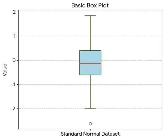 |
|---|
위 아래 T자로 나 있는 것이 수염으로 데이터 전체의 범위를 나타내준다. 그 외에 수염 부분보다 밖에 위치한 데이터는 원으로 표시한다.
도수분포표와 히스토그램
-
도수분포표
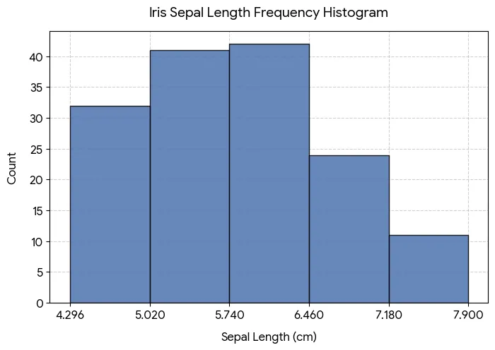
변수의 범위를 동일한 크기의 구간으로 나눈 다음, 각 구간마다 몇 개의 변숫값이 존재하는지 보여주기 위해 사용한다.
(1) 범주형 변수(species)의 도수분포표
import seaborn as sb
import pandas as pd

# Iris 데이터셋 불러오기
iris = sb.load_dataset('iris')

# species 컬럼의 도수분포표
freq_table = iris['species'].value_counts()
print(freq_table)

# 상대도수(비율) 구하기
prop_table = iris['species'].value_counts(normalize=True)
print(prop_table)
output
| class | counts |
|---|---|
| setosa | 50 |
| versicolor | 50 |
| virginica | 50 |
(2) 연속형 변수(sepal_length)의 도수분포표
# sepal_length를 5개의 구간으로 나누어 도수분포표 작성
iris['sepal_length_binned'] = pd.cut(iris['sepal_length'], bins=5)
print(iris['sepal_length_binned'].value_counts().sort_index())
output
| section | counts |
|---|---|
| (4.296, 5.02] | 32 |
| (5.02, 5.74] | 41 |
| (5.74, 6.46] | 42 |
| (6.46, 7.18] | 24 |
| (7.18, 7.9] | 11 |
구간 표시 기호 의미: 소괄호 (는 초과, 대괄호 ]는 이하를 뜻합니다. 예: (4.296, 5.02] 구간은 4.296cm 초과 ~ 5.02cm 이하인 데이터가 32개 있다는 의미
위 표에서 7.18cm-7.9cm 사이의 데이터가 적다는 분포를 볼 수 있다.
-
히스토그램
도수분포표를 시각화하는 방법이다. 범주형은 연속형이 아니기 때문에 히스토그램이 적절하지 않다.
| 연속형 변수(sepal_length)의 도수분포표 |
|---|
 |
Memorize
통계학에서는 모멘트(moment) 혹은 적률이라는 개념을 쓴다. 위치와 변이는 각각 분포의 일차 및 이차 모멘트라고 한다. 삼차, 사차 모멘트는 각각 왜도(Skewness), **첨도(kurtosis)**라고 부른다. 왜도는 데이터가 큰 값이나 작은 값 쪽으로 얼마나 비슴드히 쏠려 있는지를 나타내고, 첨도는 데이터가 극단 값을 갖는 경향성을 나타낸다. 보통을 이런 값을 직접 구하기보다는 그래프로 시각화해서 직접 확인한다.
밀도 그림과 추정
-
밀도 그림
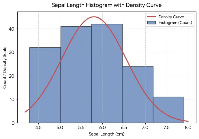
커널 밀도추정을 통해서 데이터로부터 직접 계산 한 후 보통 히스토그램 위에 데이터의 분포를 연속된 선으로 보여준다. 다른 말로 하면 부드러운 히스토그램이라고도 할 수 있다. 히스토그램과 다른 점은 y축의 값을 개수가 아닌 비율로 표시한다. 밀도 곡선 아래의 총 면적은 1이고 구간의 개수 대신 x축의 두 점 사이의 곡선 아래 면적을 계산하며, 이는 두 점 사이에 있는 분포의 비율에 해당한다.
이진 데이터와 범주 데이터 탐색하기
이진변수나 범주가 몇 개 안되는 범주형 변수는 중요한 범주의 비율만 보면 되기에 분석이 그리 어렵지 않다.
범주형 자료를 보여줄 때 주로 사용하는 것은 막대도표이다.
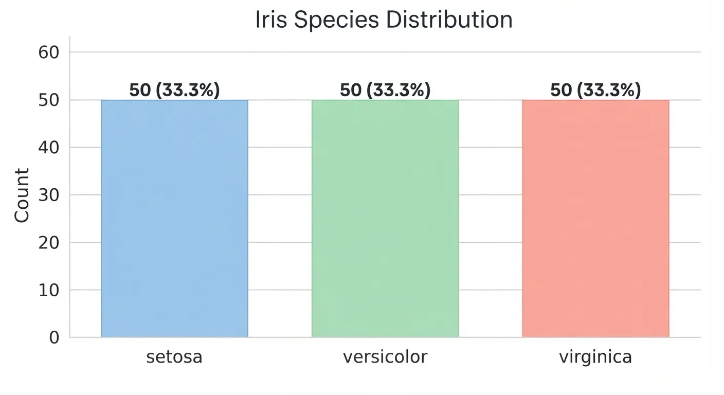 막대도표는 히스토그램과 매우 유사하다. 차이점은 x축이다. 막대 도표는 요인변수의 서로 다른 범주인 반면, 히스토그램은 수치적으로 나타낼 수 있는 하나의 변수 값을 의미한다. 그림을 보았을 때 바로 보이는 건 막대는 떨어져 있고 히스토는 붙어있다.
막대도표 대신 파이그림을 사용하기도 하지만, 시각적으로 효과적이지 않다는 이유로 잘 사용하지 않는다.
최빈값
데이터에서 가장 자주 등장하는 범주 혹은 값들.
기댓값
범주에 해당하는 어떤 수치가 있을 때, 범주의 출현 확률에 따른 평균 가중치가 해당 확률이 되는 가중평균이 기댓값이다. 이렇듯 기댓값과 가중평균과 같은 꼴이다.
import matplotlib.pyplot as plt
import seaborn as sns

# 1. 데이터 로드
df = sns.load_dataset('iris')

# 2. 품종별 평균 및 전체 평균(기준값) 계산
species_mean = df.groupby('species')['sepal_length'].mean()
overall_mean = df['sepal_length'].mean() # 5.8433...

# 3. 그래프 그리기
plt.figure(figsize=(7, 5))
bars = plt.bar(species_mean.index, species_mean.values, color=['#9ecae1', '#a1d99b', '#fcae91'], edgecolor='gray', width=0.6)

# 4. 기준값(전체 평균) 선 추가
plt.axhline(overall_mean, color='red', linestyle='--', linewidth=1.5, label=f'Overall Mean ({overall_mean:.2f} cm)')

# 5. 수치 라벨링 및 꾸미기
for bar in bars:
    height = bar.get_height()
    plt.text(bar.get_x() + bar.get_width()/2., height + 0.1, f'{height:.2f} cm', ha='center', va='bottom', fontsize=10, fontweight='bold')

plt.title('Iris Mean Sepal Length by Species', fontsize=14, pad=15)
plt.xlabel('Species', fontsize=12)
plt.ylabel('Sepal Length (cm)', fontsize=12)
plt.ylim(0, 8)
plt.legend(loc='upper left')
plt.grid(axis='y', linestyle=':', alpha=0.6)

plt.tight_layout()
plt.show()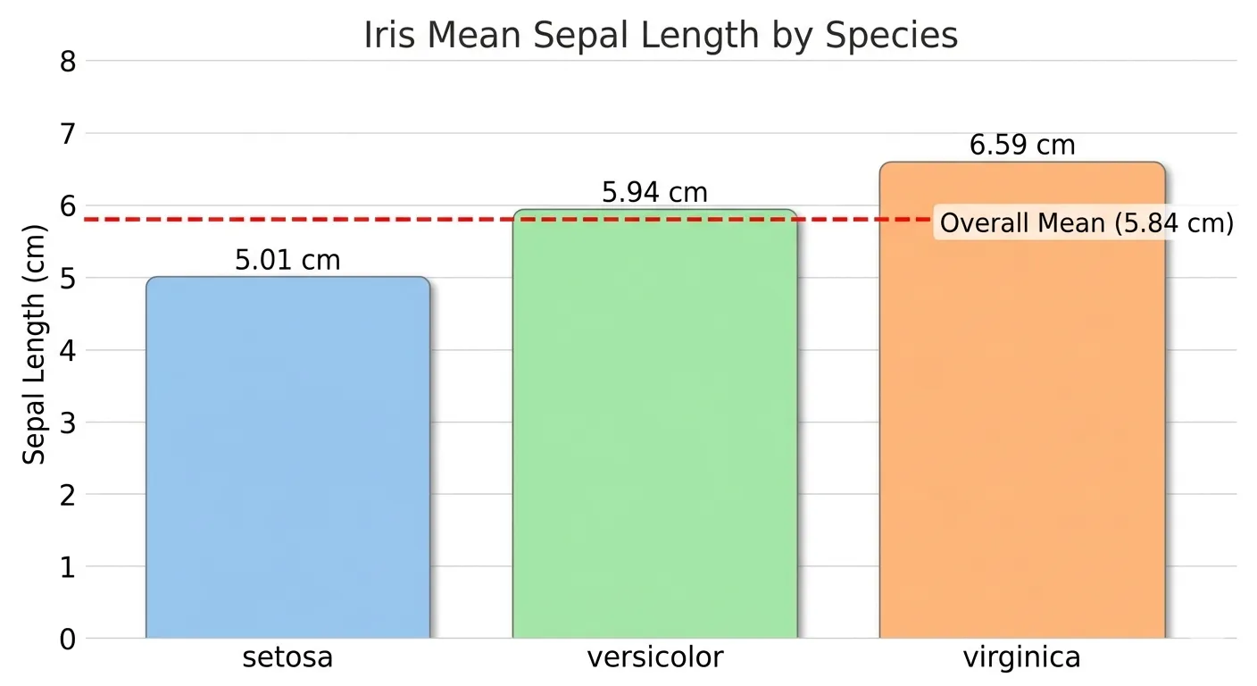
Misleading graph
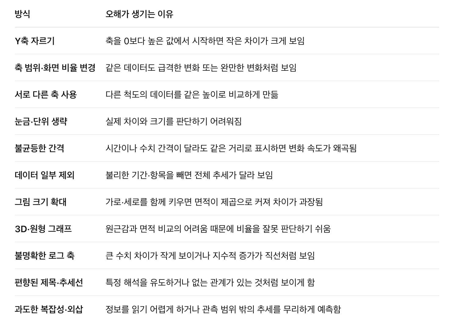 왜곡 정도를 나타내는 대표 지표는 Lie factor이다.
확률
사건이 발생할 확률이란 상황이 수없이 반복될 경우 사건이 발생할 비율을 의미.
*어떻게 정의하는가에 따라 철학적 토론할 수밖에 없지만, 이 책은 위와 같은 의미로 정의한다.
상관관계
**탐색적 데이터 분석(EDA)**을 하는 과정에서 예측값과 목푯값과의 상관관계를 조사해야 한다. 가 큰 값을 가질 때 가 큰 값을 가지고, 가 작은 값을 가질 때 가 작은 값을 가지는 경우 서로 양의 상관관계를 가진다. 반대로 가 큰 값을 가질 때 가 작은 값을 가지는 경우에는 음의 상관관계를 가진다.
- 상관계수(correlation coefficien): 수치적 변수들 간에 어떤 관계가 있는지 나타내기 위해 사용되는 측정량(-1에서 +1까지의 범위)
- 상관행렬(correlation matrix): 행과 열이 변수들을 의미하는 표를 말하며, 각 셀은 그 행과 열에 해당하는 변수들 간의 상관관계를 의미한다.
아래 변수 볼 때 벡터곱합은 32이다.
- v1: {1, 2, 3}
- v2: {4, 5, 6}
벡터의 순서를 섞어서 곱해서 더해도 32를 넘을 수 없다. 즉 32라는 합을 랜덤으로 섞었을 때 나오는 값들과 비교해볼 수 있을 것이다. 하지만 이런 값들은 재표본분포에 대한 레퍼런스로서의 의미밖에는 없다.
- 재표본분포(Resampling Distribution): 관측된 데이터나 표본에서 반복적으로(복원 또는 비복원) 데이터를 추출해 만든 통계량(평균, 중앙값, 차이 등)의 확률 분포
이런 방법보다는 상관계수(피어슨 상관계수라고도 함)라는 표준화된 방식이 훨씬 더 유용하다.
의미
| 기호 | 의미 |
|---|---|
| 데이터 쌍의 개수 | |
| 번째 데이터 쌍 | |
| 각 변수의 평균 | |
| 각 변수의 표본 표준편차 |
해석
| 값 | 해석 |
|---|---|
| 에 가까움 | 가 커질수록 도 커지는 강한 직선적 관계 |
| 에 가까움 | 직선적 관계가 약함 |
| 에 가까움 | 가 커질수록 는 작아지는 강한 직선적 관계 |
두 변수 간의 선형적인 관계를 갖지 않을 경우, 상관계수는 유용한 측정 지표가 아니다.
import matplotlib.pyplot as plt
import seaborn as sns
import pandas as pd
from sklearn.datasets import load_iris

# 1. 데이터 불러오기 및 깔끔한 변수명 설정
iris = load_iris()
df = pd.DataFrame(iris.data, columns=['Sepal Length', 'Sepal Width', 'Petal Length', 'Petal Width'])
corr_matrix = df.corr()

# 2. 히트맵 시각화
plt.figure(figsize=(8, 6))
sns.heatmap(
    corr_matrix,
    annot=True,          # 수치 표시
    cmap='RdBu_r',       # 양수: 빨강, 음수: 파랑 (0: 흰색)
    vmin=-1,             # 최소-최대 고정으로 0의 기준점 유지
    vmax=1,
    center=0,
    fmt='.2f',           # 소수점 둘째 자리
    linewidths=0.5,      # 셀 사이 선 두께
    cbar_kws={"shrink": 0.8}
)

plt.title('Iris Feature Correlation Heatmap', fontsize=14, pad=15)
plt.tight_layout()

# 3. PNG 파일로 저장 (고해상도 150 DPI)
plt.savefig('iris_heatmap.png', dpi=150)
plt.show()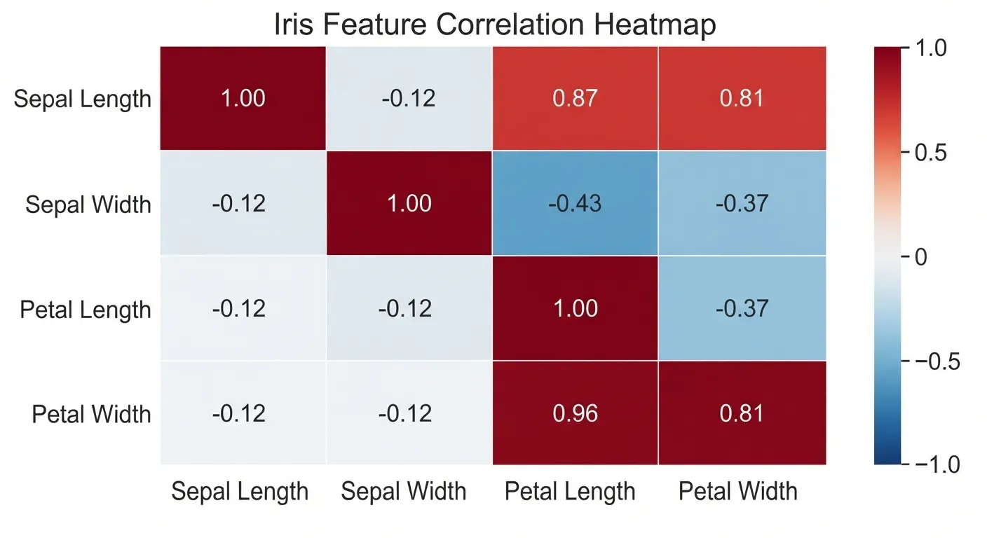
*상관계수는 특잇값에 민감하다.
산점도
축과 축이 서로 다른 두 개의 변수를 나타내는 도표 두 변수 사이의 관계를 시각화하는 가장 기본적인 방법이 산점도를 그려보는 것이다.
import matplotlib.pyplot as plt
from sklearn.datasets import load_iris

iris = load_iris()

for i, species in enumerate(iris.target_names):
    mask = iris.target == i
    plt.scatter(
        iris.data[mask, 2],
        iris.data[mask, 3],
        label=species,
        alpha=0.8
    )

plt.xlabel("Petal Length (cm)")
plt.ylabel("Petal Width (cm)")
plt.title("Iris: Petal Length vs. Petal Width")
plt.legend(title="Species")
plt.grid(alpha=0.2)
plt.tight_layout()
plt.savefig("petal_scatter.png", dpi=200)
plt.show()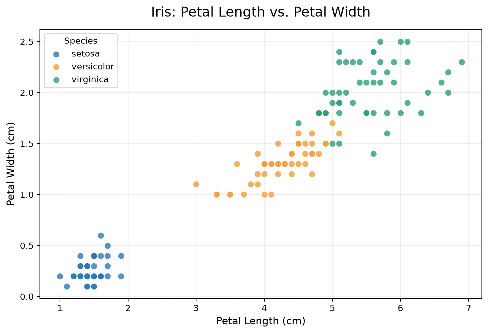
두 개 이상의 변수 탐색하기
평균과 분산과 같이 익숙한 추정값은 일변량분석(한 번에 하나의 변수), 상관분석은 이변량분석, 셋 이상의 변수를 분석하는 것을 다변량분석이라고 한다.
- 분할표(Contingency Table): 두 가지 이상의 범주형 변수의 빈도수를 기록한 표
- 육각형 구간(Hexagonal Binning): 두 변수를 육각형 모양의 구간으로 나눈 그림
- 등고 도표(Contour Plot): 지도상에 같은 높이의 지점을 등고선으로 나타내는 것처럼, 두 변수의 밀도를 등고선으로 표시한 도표
- 바이올린 도표(Violin Plot): 상자그림과 비슷하지만 밀도추정을 함께 보여준다.
육각형 구간과 등고선(수치형 변수 대 수치형 변수를 시각화)
산점도는 데이터의 개수가 상대적으로 적을 때는 괜찮지만, 수백만의 레코드를 나타내기에는 점들이 너무 밀집되어 알아보기 어렵다. 그럴 때 아래와 같은 육각형 구간
import matplotlib.pyplot as plt
import seaborn as sns

# 1. 붓꽃(Iris) 내장 데이터셋 로드
iris = sns.load_dataset('iris')

# 데이터 추출
x = iris['petal_length']
y = iris['petal_width']

# 2. 그래프 크기 설정 및 hexbin 플롯 그리기
plt.figure(figsize=(9, 6))

# gridsize: 육각형의 크기/조밀도 조정
# cmap: 'viridis' 컬러맵 적용 (기본값)
# mincnt: 데이터가 1개 이상 있는 빈(bin)만 표시하여 빈 곳을 흰색으로 처리
hb = plt.hexbin(x, y, gridsize=20, cmap='viridis', mincnt=1)

# 3. 우측 컬러바(Colorbar) 추가 및 라벨 설정
cb = plt.colorbar(hb)
cb.set_label('Number of samples')

# 4. 타이틀 및 축 라벨 설정
plt.title('Iris: Petal Length vs. Petal Width (Hexbin)', fontsize=14, pad=15)
plt.xlabel('Petal Length (cm)', fontsize=12)
plt.ylabel('Petal Width (cm)', fontsize=12)

# 5. 축 눈금 및 범위 세부 조정 (이미지와 일치하도록 설정)
plt.xlim(0.5, 7.5)
plt.ylim(-0.1, 2.6)

# 그래프 표시
plt.tight_layout()
plt.show()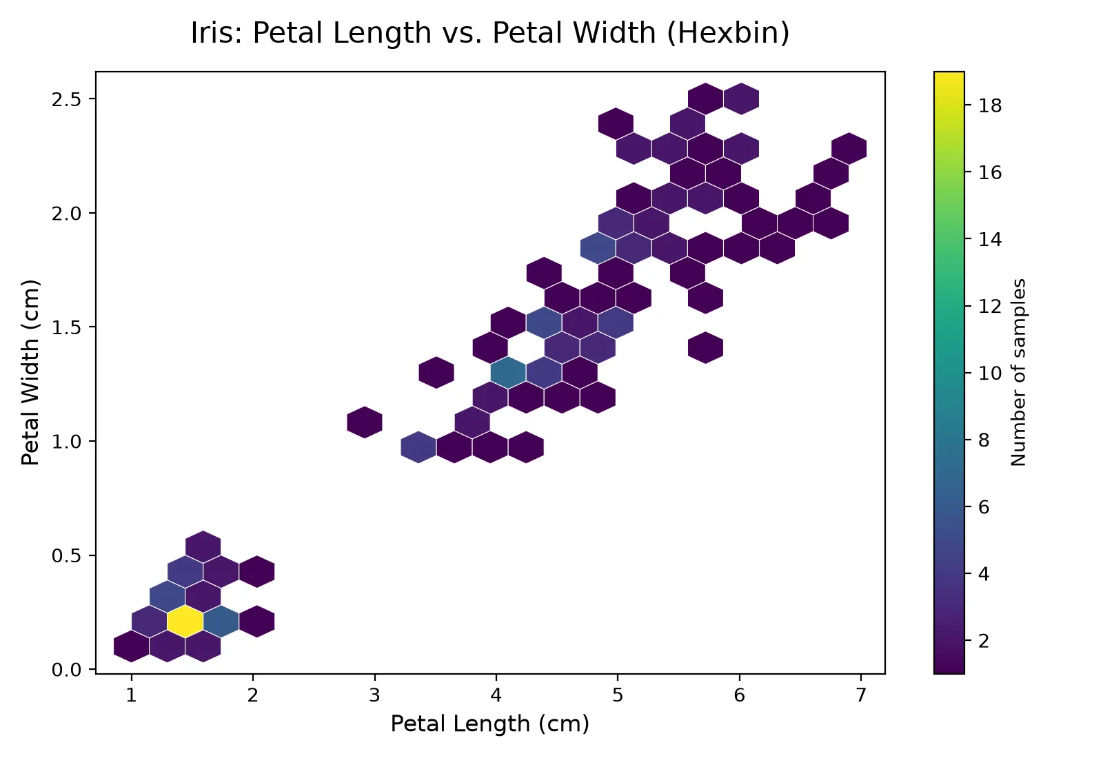
등고선은 꼭대기 쪽으로 갈수록 밀도가 높아진다.
import matplotlib.pyplot as plt
import seaborn as sns

# 1. 붓꽃(Iris) 데이터셋 로드
iris = sns.load_dataset('iris')

plt.figure(figsize=(9, 6))

# 2. 등고선 그래프(KDE Plot) 그리기
# fill=True를 주면 등고선 사이가 색상으로 채워집니다.
sns.kdeplot(
    data=iris,
    x='petal_length',
    y='petal_width',
    cmap='viridis',    # 육각형 그래프와 동일한 컬러맵 적용
    fill=True,         # 등고선 내부 채우기 (선만 그리려면 False)
    thresh=0.05,       # 밀도가 아주 낮은 외곽 영역 제거
    levels=10          # 등고선 층의 개수
)

# 3. 타이틀 및 축 라벨 설정
plt.title('Iris: Petal Length vs. Petal Width (Contour/KDE)', fontsize=14, pad=15)
plt.xlabel('Petal Length (cm)', fontsize=12)
plt.ylabel('Petal Width (cm)', fontsize=12)

# 4. 축 범위 조정
plt.xlim(0.5, 7.5)
plt.ylim(-0.1, 2.6)

plt.tight_layout()
plt.show()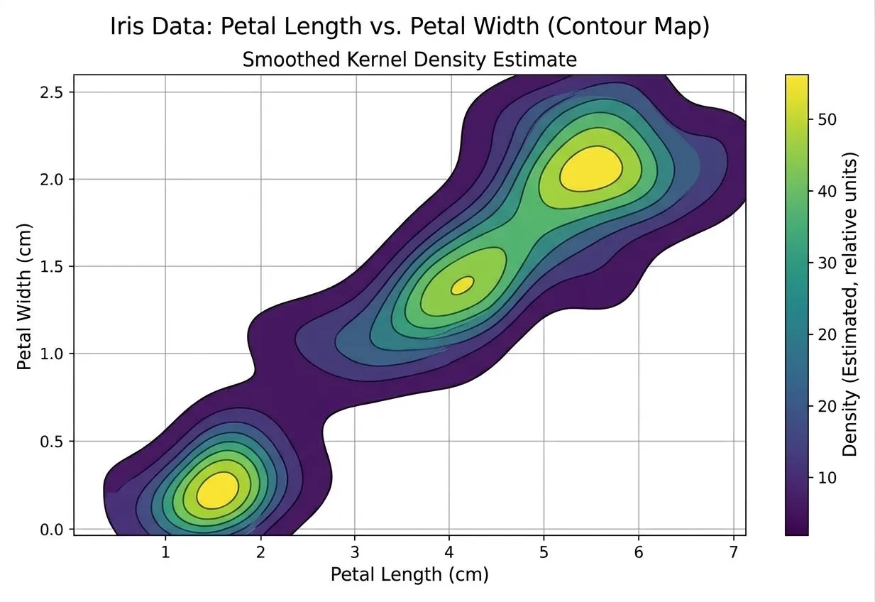
두 수치형 변수의 관계를 나타내는 다른 도표로 히트맵이 있다.
import matplotlib.pyplot as plt
import numpy as np

# 색상 값과 셀에 표시할 문구를 별도로 지정
colors = np.array([
    [0.09, 0.60, 0.00, 0.13],
    [0.44, 0.67, 0.16, 0.59],
    [0.92, 1.00, 0.20, 0.96],
])

labels = [
    ["1.46 cm", "1.46 cm", "0.69 cm", "0.78 Corr"],
    ["11.37 cm", "12.25 cm", "1.03 cm", "0.79 Corr"],
    ["1.46 cm", "0.78 Corr", "1.01 cm", "0.73 Corr"],
]

species = ["Setosa", "Versicolor", "Virginica"]
variables = [
    "Petal Length [Low]",
    "Petal Length [High]",
    "Petal Width [Low]",
    "Petal Width [High]",
]

fig, ax = plt.subplots(figsize=(14, 9))

heatmap = ax.imshow(
    colors,
    cmap="viridis",
    vmin=0,
    vmax=1,
    aspect="auto",
    interpolation="nearest",
)

ax.set_xticks(np.arange(len(variables)), labels=variables)
ax.set_yticks(np.arange(len(species)), labels=species)
ax.tick_params(axis="both", labelsize=14)

ax.set_xlabel("Variable Group", fontsize=20)
ax.set_ylabel("Species", fontsize=20)
ax.set_title(
    "Iris Data Analysis (Heatmap)\n"
    "Correlation and Mean Values Matrix",
    fontsize=25,
    pad=12,
)

# 셀 사이 흰색 구분선
ax.set_xticks(np.arange(0.5, 3.5, 1), minor=True)
ax.set_yticks(np.arange(0.5, 2.5, 1), minor=True)
ax.grid(which="minor", color="white", linewidth=2)
ax.tick_params(which="minor", bottom=False, left=False)

# 셀 내부 문구
for row in range(len(species)):
    for col in range(len(variables)):
        ax.text(
            col,
            row,
            labels[row][col],
            ha="center",
            va="center",
            fontsize=21,
            color="#171717" if colors[row, col] > 0.8 else "#eeeeee",
        )

colorbar = fig.colorbar(
    heatmap,
    ax=ax,
    ticks=np.linspace(0, 1, 6),
    fraction=0.04,
    pad=0.07,
)
colorbar.ax.tick_params(labelsize=16)
colorbar.set_label(
    "Normalized Mean or Correlation Value\n(Arbitrary Units)",
    fontsize=20,
)

plt.tight_layout()
plt.show()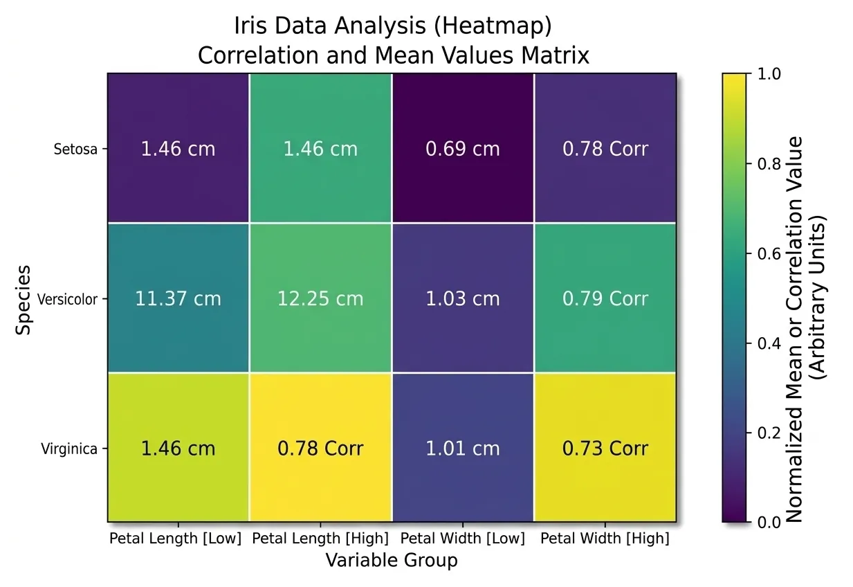
범주형 변수 대 범주형 변수
분할표는 두 범주형 변수를 요약하는 데 효과적인 방법, 범주별 빈도수를 기록한 표다.
꽃받침 길이(중간값 기준) 분할표
import pandas as pd
from sklearn.datasets import load_iris

# 1. 아이리스 데이터셋 로드
iris = load_iris()
df = pd.DataFrame(iris.data, columns=iris.feature_names)

# 타겟(품종) 데이터 추가 및 문자열 이름 매핑 ('setosa', 'versicolor', 'virginica')
df['species'] = [iris.target_names[t] for t in iris.target]

# 2. 연속형 변수 하나를 범주형 변수로 변환 (예: 꽃받침 길이를 중간값 기준으로 Short/Long 분할)
df['sepal_length_cat'] = pd.qcut(df['sepal length (cm)'], q=2, labels=['Short', 'Long'])

# 3. 두 범주형 변수('sepal_length_cat'과 'species')로 분할표 생성
contingency_table = pd.crosstab(index=df['sepal_length_cat'], columns=df['species'])

# 결과 출력
print(contingency_table)
결과 출력
| sepal_length_cat | setosa | versicolor | virginica |
|---|---|---|---|
| Short | 47 | 24 | 10 |
| Long | 3 | 26 | 40 |
범주형 변수 대 수치형 변수
상자그림이 범주형 변수에 따라 분류된 수치형 변수의 분포를 시각화하여 비교하는 간단한 방법이다.
import matplotlib.pyplot as plt
import seaborn as sns

# 1. Seaborn의 내장 내장 iris 데이터셋 로드
iris = sns.load_dataset("iris")

# 한글 깨짐 방지 설정 (필요한 경우 주석 해제 후 사용)
# plt.rc('font', family='Malgun Gothic') # Windows
# plt.rc('font', family='AppleGothic') # Mac
# plt.rcParams['axes.unicode_minus'] = False

# 2. 그래프 크기 설정
plt.figure(figsize=(8, 6))

# 3. 클래스(species)별 꽃잎 길이(petal_length) 상자그림 그리기
sns.boxplot(x="species", y="petal_length", data=iris, palette="Set2")

# 4. 그래프 제목 및 축 레이블 설정
plt.title("Boxplot of Petal Length by Iris Species", fontsize=14)
plt.xlabel("Species (품종)", fontsize=12)
plt.ylabel("Petal Length (꽃잎 길이)", fontsize=12)

# 5. 그래프 출력
plt.show()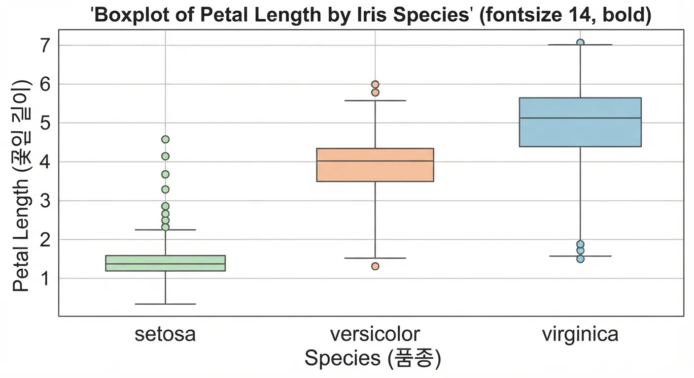
import matplotlib.pyplot as plt
import seaborn as sns

# 1. Seaborn의 내장 iris 데이터셋 로드
iris = sns.load_dataset("iris")

# 한글 깨짐 방지 설정 (필요한 경우 주석 해제 후 사용)
# plt.rc('font', family='Malgun Gothic') # Windows
# plt.rc('font', family='AppleGothic') # Mac
# plt.rcParams['axes.unicode_minus'] = False

# 2. 그래프 크기 설정
plt.figure(figsize=(8, 6))

# 3. 클래스(species)별 꽃잎 길이(petal_length) 바이올린 도표 그리기
# inner="box"를 설정하면 바이올린 내부에 작은 상자그림이 함께 그려집니다.
sns.violinplot(x="species", y="petal_length", data=iris, palette="Set2", inner="box")

# 4. 그래프 제목 및 축 레이블 설정
plt.title("Violin Plot of Petal Length by Iris Species", fontsize=14)
plt.xlabel("Species (품종)", fontsize=12)
plt.ylabel("Petal Length (꽃잎 길이)", fontsize=12)

# 5. 그래프 출력
plt.show()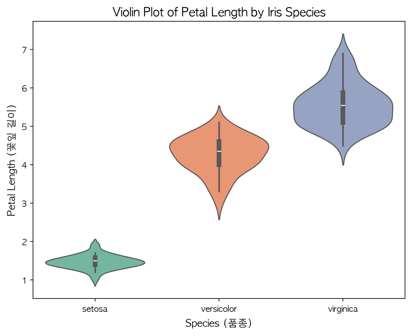
다변수 시각화하기
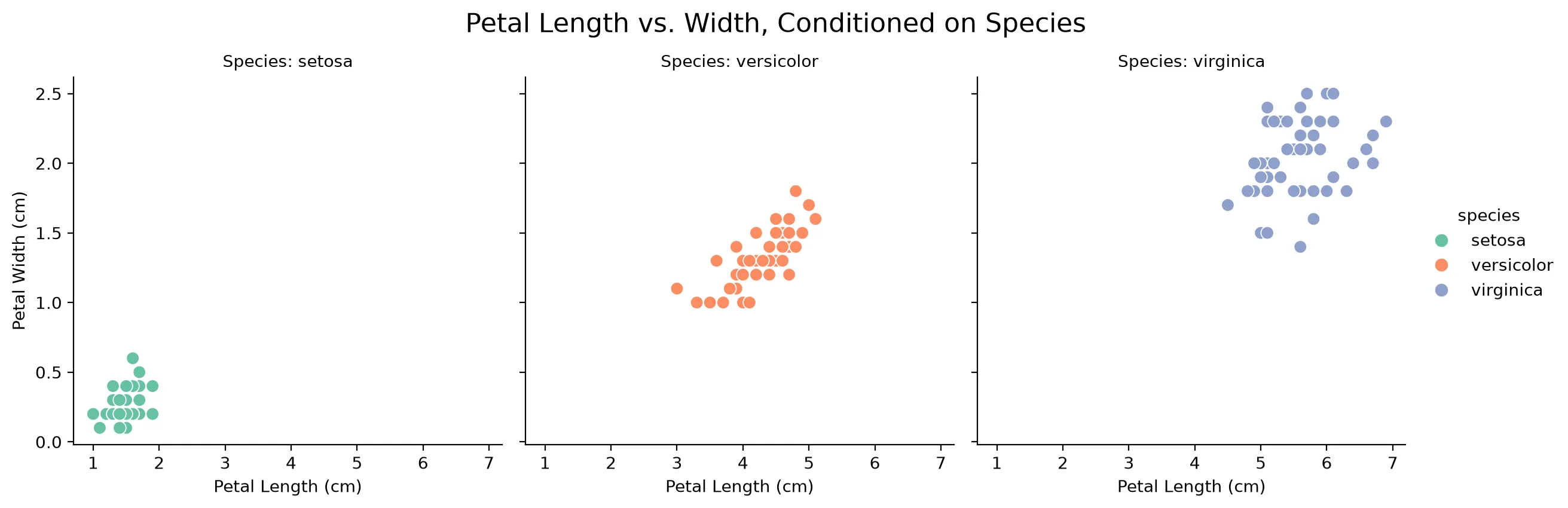
조건화라는 개념을 통해 두 변수 비교용 도표를 더 여러 변수를 비교하는 용도로 확장하여 활용할 수도 있다.
Exploring the data distribution
Percentiles and boxplots
-
Percentiles
Percentiles are what we usually use to understand the whole distribution. The most common are quartiles (the 25th, 50th and 75th percentiles) and deciles (the 10th, 20th, 30th, …, 90th percentiles). They are good for describing the tails (the outer range).
-
Boxplots
An easy way to visualize the spread of data using percentiles.
import matplotlib.pyplot as plt
import numpy as np

# 가상 데이터 생성
data = np.random.randn(100)

# 박스 플롯 그리기
plt.figure(figsize=(6, 4))
plt.boxplot(data)
plt.title("Basic Box Plot")
plt.show() |
|---|
The T-shaped lines above and below are the whiskers, which show the range of the data. Data that falls outside the whiskers is shown as circles.
Frequency tables and histograms
-
Frequency tables
Used to divide a variable’s range into equal-sized intervals and show how many values fall into each interval.
(1) Frequency table of a categorical variable (species)
import seaborn as sb
import pandas as pd

# Iris 데이터셋 불러오기
iris = sb.load_dataset('iris')

# species 컬럼의 도수분포표
freq_table = iris['species'].value_counts()
print(freq_table)

# 상대도수(비율) 구하기
prop_table = iris['species'].value_counts(normalize=True)
print(prop_table)
output
| class | counts |
|---|---|
| setosa | 50 |
| versicolor | 50 |
| virginica | 50 |
(2) Frequency table of a continuous variable (sepal_length)
# sepal_length를 5개의 구간으로 나누어 도수분포표 작성
iris['sepal_length_binned'] = pd.cut(iris['sepal_length'], bins=5)
print(iris['sepal_length_binned'].value_counts().sort_index())
output
| section | counts |
|---|---|
| (4.296, 5.02] | 32 |
| (5.02, 5.74] | 41 |
| (5.74, 6.46] | 42 |
| (6.46, 7.18] | 24 |
| (7.18, 7.9] | 11 |
What the interval brackets mean: a parenthesis ( means “greater than” and a square bracket ] means “less than or equal to”. For example, the interval (4.296, 5.02] means there are 32 data points greater than 4.296cm and at most 5.02cm
The table above shows that there is little data between 7.18cm and 7.9cm.
-
Histograms
A way to visualize a frequency table. Categorical data is not continuous, so a histogram is not appropriate for it.
| Frequency table of a continuous variable (sepal_length) |
|---|
|
Memorize
Statistics uses the concept of moments. Location and variability are called the first and second moments of a distribution. The third and fourth moments are called skewness and kurtosis. Skewness indicates how much the data leans toward larger or smaller values, and kurtosis indicates the tendency of the data to have extreme values. Usually, rather than computing these values directly, we check them visually with plots.
Density plots and estimation
-
Density plots
Computed directly from the data through kernel density estimation, usually shown as a continuous line over a histogram. In other words, it can be called a smoothed histogram. Unlike a histogram, the y-axis shows proportions rather than counts. The total area under the density curve is 1, and instead of counts per interval you compute the area under the curve between two points on the x-axis, which corresponds to the proportion of the distribution between those points.
Exploring binary and categorical data
For binary variables, or categorical variables with only a few categories, you only need to look at the proportions of the important categories, so the analysis is not difficult.
The bar chart is the most common way to show categorical data.
A bar chart is very similar to a histogram. The difference is the x-axis. In a bar chart it represents the different categories of a factor variable, while in a histogram it represents the values of a single numeric variable. The visible difference is that bars are separated while histogram bins touch.
Pie charts are sometimes used instead of bar charts, but they are rarely used because they are visually less effective.
Mode
The category or value that appears most often in the data.
Expected value
When categories have numeric values attached, the average weighted by the probability of each category occurring. The expected value is a weighted mean whose weights are those probabilities. In this sense, the expected value has the same form as a weighted mean.
import matplotlib.pyplot as plt
import seaborn as sns

# 1. 데이터 로드
df = sns.load_dataset('iris')

# 2. 품종별 평균 및 전체 평균(기준값) 계산
species_mean = df.groupby('species')['sepal_length'].mean()
overall_mean = df['sepal_length'].mean() # 5.8433...

# 3. 그래프 그리기
plt.figure(figsize=(7, 5))
bars = plt.bar(species_mean.index, species_mean.values, color=['#9ecae1', '#a1d99b', '#fcae91'], edgecolor='gray', width=0.6)

# 4. 기준값(전체 평균) 선 추가
plt.axhline(overall_mean, color='red', linestyle='--', linewidth=1.5, label=f'Overall Mean ({overall_mean:.2f} cm)')

# 5. 수치 라벨링 및 꾸미기
for bar in bars:
    height = bar.get_height()
    plt.text(bar.get_x() + bar.get_width()/2., height + 0.1, f'{height:.2f} cm', ha='center', va='bottom', fontsize=10, fontweight='bold')

plt.title('Iris Mean Sepal Length by Species', fontsize=14, pad=15)
plt.xlabel('Species', fontsize=12)
plt.ylabel('Sepal Length (cm)', fontsize=12)
plt.ylim(0, 8)
plt.legend(loc='upper left')
plt.grid(axis='y', linestyle=':', alpha=0.6)

plt.tight_layout()
plt.show()
Misleading graph
The representative measure of how much a graph distorts is the Lie factor.
Probability
The probability of an event is the proportion of times the event would occur if the situation were repeated countless times.
*How to define it inevitably leads to philosophical debate, but this book defines it as above.
Correlation
During exploratory data analysis (EDA), you need to examine the correlation between predictors and the target. When tends to be large when is large, and small when is small, they have a positive correlation. Conversely, when tends to be small when is large, they have a negative correlation.
- Correlation coefficient: a metric used to show how numeric variables relate to each other (ranging from -1 to +1)
- Correlation matrix: a table whose rows and columns are variables, where each cell is the correlation between the variables of that row and column.
For the variables below, the sum of the element-wise products is 32.
- v1: {1, 2, 3}
- v2: {4, 5, 6}
No matter how you shuffle the order of the vectors before multiplying and summing, you cannot exceed 32. So you could compare the sum of 32 against the values you get from random shuffles. But such values only serve as a reference for a resampling distribution.
- Resampling distribution: the probability distribution of a statistic (mean, median, difference, etc.) built by repeatedly drawing data (with or without replacement) from the observed data or sample
A standardized measure called the correlation coefficient (also known as Pearson’s correlation coefficient) is far more useful than this approach.
Meaning
| Symbol | Meaning |
|---|---|
| Number of data pairs | |
| The -th data pair | |
| Mean of each variable | |
| Sample standard deviation of each variable |
Interpretation
| Value of | Interpretation |
|---|---|
| Close to | A strong linear relationship where increases as increases |
| Close to | A weak linear relationship |
| Close to | A strong linear relationship where decreases as increases |
When two variables do not have a linear relationship, the correlation coefficient is not a useful metric.
import matplotlib.pyplot as plt
import seaborn as sns
import pandas as pd
from sklearn.datasets import load_iris

# 1. 데이터 불러오기 및 깔끔한 변수명 설정
iris = load_iris()
df = pd.DataFrame(iris.data, columns=['Sepal Length', 'Sepal Width', 'Petal Length', 'Petal Width'])
corr_matrix = df.corr()

# 2. 히트맵 시각화
plt.figure(figsize=(8, 6))
sns.heatmap(
    corr_matrix,
    annot=True,          # 수치 표시
    cmap='RdBu_r',       # 양수: 빨강, 음수: 파랑 (0: 흰색)
    vmin=-1,             # 최소-최대 고정으로 0의 기준점 유지
    vmax=1,
    center=0,
    fmt='.2f',           # 소수점 둘째 자리
    linewidths=0.5,      # 셀 사이 선 두께
    cbar_kws={"shrink": 0.8}
)

plt.title('Iris Feature Correlation Heatmap', fontsize=14, pad=15)
plt.tight_layout()

# 3. PNG 파일로 저장 (고해상도 150 DPI)
plt.savefig('iris_heatmap.png', dpi=150)
plt.show()
*The correlation coefficient is sensitive to outliers.
Scatterplots
A plot whose -axis and -axis represent two different variables The most basic way to visualize the relationship between two variables is to draw a scatterplot.
import matplotlib.pyplot as plt
from sklearn.datasets import load_iris

iris = load_iris()

for i, species in enumerate(iris.target_names):
    mask = iris.target == i
    plt.scatter(
        iris.data[mask, 2],
        iris.data[mask, 3],
        label=species,
        alpha=0.8
    )

plt.xlabel("Petal Length (cm)")
plt.ylabel("Petal Width (cm)")
plt.title("Iris: Petal Length vs. Petal Width")
plt.legend(title="Species")
plt.grid(alpha=0.2)
plt.tight_layout()
plt.savefig("petal_scatter.png", dpi=200)
plt.show()
Exploring two or more variables
Familiar estimates like the mean and variance are univariate analysis (one variable at a time), correlation analysis is bivariate analysis, and analyzing three or more variables is called multivariate analysis.
- Contingency table: a table recording the counts of two or more categorical variables
- Hexagonal binning: a plot that divides two variables into hexagon-shaped bins
- Contour plot: a plot that shows the density of two variables with contour lines, like a map showing points of equal elevation with contour lines
- Violin plot: similar to a boxplot, but also shows a density estimate.
Hexagonal binning and contours (numeric vs numeric)
Scatterplots work when there are relatively few data points, but for millions of records the points are too dense to read. In that case, hexagonal binning like the one below
import matplotlib.pyplot as plt
import seaborn as sns

# 1. 붓꽃(Iris) 내장 데이터셋 로드
iris = sns.load_dataset('iris')

# 데이터 추출
x = iris['petal_length']
y = iris['petal_width']

# 2. 그래프 크기 설정 및 hexbin 플롯 그리기
plt.figure(figsize=(9, 6))

# gridsize: 육각형의 크기/조밀도 조정
# cmap: 'viridis' 컬러맵 적용 (기본값)
# mincnt: 데이터가 1개 이상 있는 빈(bin)만 표시하여 빈 곳을 흰색으로 처리
hb = plt.hexbin(x, y, gridsize=20, cmap='viridis', mincnt=1)

# 3. 우측 컬러바(Colorbar) 추가 및 라벨 설정
cb = plt.colorbar(hb)
cb.set_label('Number of samples')

# 4. 타이틀 및 축 라벨 설정
plt.title('Iris: Petal Length vs. Petal Width (Hexbin)', fontsize=14, pad=15)
plt.xlabel('Petal Length (cm)', fontsize=12)
plt.ylabel('Petal Width (cm)', fontsize=12)

# 5. 축 눈금 및 범위 세부 조정 (이미지와 일치하도록 설정)
plt.xlim(0.5, 7.5)
plt.ylim(-0.1, 2.6)

# 그래프 표시
plt.tight_layout()
plt.show()
In a contour plot, density increases toward the peaks.
import matplotlib.pyplot as plt
import seaborn as sns

# 1. 붓꽃(Iris) 데이터셋 로드
iris = sns.load_dataset('iris')

plt.figure(figsize=(9, 6))

# 2. 등고선 그래프(KDE Plot) 그리기
# fill=True를 주면 등고선 사이가 색상으로 채워집니다.
sns.kdeplot(
    data=iris,
    x='petal_length',
    y='petal_width',
    cmap='viridis',    # 육각형 그래프와 동일한 컬러맵 적용
    fill=True,         # 등고선 내부 채우기 (선만 그리려면 False)
    thresh=0.05,       # 밀도가 아주 낮은 외곽 영역 제거
    levels=10          # 등고선 층의 개수
)

# 3. 타이틀 및 축 라벨 설정
plt.title('Iris: Petal Length vs. Petal Width (Contour/KDE)', fontsize=14, pad=15)
plt.xlabel('Petal Length (cm)', fontsize=12)
plt.ylabel('Petal Width (cm)', fontsize=12)

# 4. 축 범위 조정
plt.xlim(0.5, 7.5)
plt.ylim(-0.1, 2.6)

plt.tight_layout()
plt.show()
Another plot that shows the relationship between two numeric variables is the heatmap.
import matplotlib.pyplot as plt
import numpy as np

# 색상 값과 셀에 표시할 문구를 별도로 지정
colors = np.array([
    [0.09, 0.60, 0.00, 0.13],
    [0.44, 0.67, 0.16, 0.59],
    [0.92, 1.00, 0.20, 0.96],
])

labels = [
    ["1.46 cm", "1.46 cm", "0.69 cm", "0.78 Corr"],
    ["11.37 cm", "12.25 cm", "1.03 cm", "0.79 Corr"],
    ["1.46 cm", "0.78 Corr", "1.01 cm", "0.73 Corr"],
]

species = ["Setosa", "Versicolor", "Virginica"]
variables = [
    "Petal Length [Low]",
    "Petal Length [High]",
    "Petal Width [Low]",
    "Petal Width [High]",
]

fig, ax = plt.subplots(figsize=(14, 9))

heatmap = ax.imshow(
    colors,
    cmap="viridis",
    vmin=0,
    vmax=1,
    aspect="auto",
    interpolation="nearest",
)

ax.set_xticks(np.arange(len(variables)), labels=variables)
ax.set_yticks(np.arange(len(species)), labels=species)
ax.tick_params(axis="both", labelsize=14)

ax.set_xlabel("Variable Group", fontsize=20)
ax.set_ylabel("Species", fontsize=20)
ax.set_title(
    "Iris Data Analysis (Heatmap)\n"
    "Correlation and Mean Values Matrix",
    fontsize=25,
    pad=12,
)

# 셀 사이 흰색 구분선
ax.set_xticks(np.arange(0.5, 3.5, 1), minor=True)
ax.set_yticks(np.arange(0.5, 2.5, 1), minor=True)
ax.grid(which="minor", color="white", linewidth=2)
ax.tick_params(which="minor", bottom=False, left=False)

# 셀 내부 문구
for row in range(len(species)):
    for col in range(len(variables)):
        ax.text(
            col,
            row,
            labels[row][col],
            ha="center",
            va="center",
            fontsize=21,
            color="#171717" if colors[row, col] > 0.8 else "#eeeeee",
        )

colorbar = fig.colorbar(
    heatmap,
    ax=ax,
    ticks=np.linspace(0, 1, 6),
    fraction=0.04,
    pad=0.07,
)
colorbar.ax.tick_params(labelsize=16)
colorbar.set_label(
    "Normalized Mean or Correlation Value\n(Arbitrary Units)",
    fontsize=20,
)

plt.tight_layout()
plt.show()
Categorical vs categorical
A contingency table is an effective way to summarize two categorical variables: a table that records the counts for each combination of categories.
Contingency table of sepal length (split at the median)
import pandas as pd
from sklearn.datasets import load_iris

# 1. 아이리스 데이터셋 로드
iris = load_iris()
df = pd.DataFrame(iris.data, columns=iris.feature_names)

# 타겟(품종) 데이터 추가 및 문자열 이름 매핑 ('setosa', 'versicolor', 'virginica')
df['species'] = [iris.target_names[t] for t in iris.target]

# 2. 연속형 변수 하나를 범주형 변수로 변환 (예: 꽃받침 길이를 중간값 기준으로 Short/Long 분할)
df['sepal_length_cat'] = pd.qcut(df['sepal length (cm)'], q=2, labels=['Short', 'Long'])

# 3. 두 범주형 변수('sepal_length_cat'과 'species')로 분할표 생성
contingency_table = pd.crosstab(index=df['sepal_length_cat'], columns=df['species'])

# 결과 출력
print(contingency_table)
Output
| sepal_length_cat | setosa | versicolor | virginica |
|---|---|---|---|
| Short | 47 | 24 | 10 |
| Long | 3 | 26 | 40 |
Categorical vs numeric
A boxplot is a simple way to visually compare the distribution of a numeric variable grouped by a categorical variable.
import matplotlib.pyplot as plt
import seaborn as sns

# 1. Seaborn의 내장 내장 iris 데이터셋 로드
iris = sns.load_dataset("iris")

# 한글 깨짐 방지 설정 (필요한 경우 주석 해제 후 사용)
# plt.rc('font', family='Malgun Gothic') # Windows
# plt.rc('font', family='AppleGothic') # Mac
# plt.rcParams['axes.unicode_minus'] = False

# 2. 그래프 크기 설정
plt.figure(figsize=(8, 6))

# 3. 클래스(species)별 꽃잎 길이(petal_length) 상자그림 그리기
sns.boxplot(x="species", y="petal_length", data=iris, palette="Set2")

# 4. 그래프 제목 및 축 레이블 설정
plt.title("Boxplot of Petal Length by Iris Species", fontsize=14)
plt.xlabel("Species (품종)", fontsize=12)
plt.ylabel("Petal Length (꽃잎 길이)", fontsize=12)

# 5. 그래프 출력
plt.show()
import matplotlib.pyplot as plt
import seaborn as sns

# 1. Seaborn의 내장 iris 데이터셋 로드
iris = sns.load_dataset("iris")

# 한글 깨짐 방지 설정 (필요한 경우 주석 해제 후 사용)
# plt.rc('font', family='Malgun Gothic') # Windows
# plt.rc('font', family='AppleGothic') # Mac
# plt.rcParams['axes.unicode_minus'] = False

# 2. 그래프 크기 설정
plt.figure(figsize=(8, 6))

# 3. 클래스(species)별 꽃잎 길이(petal_length) 바이올린 도표 그리기
# inner="box"를 설정하면 바이올린 내부에 작은 상자그림이 함께 그려집니다.
sns.violinplot(x="species", y="petal_length", data=iris, palette="Set2", inner="box")

# 4. 그래프 제목 및 축 레이블 설정
plt.title("Violin Plot of Petal Length by Iris Species", fontsize=14)
plt.xlabel("Species (품종)", fontsize=12)
plt.ylabel("Petal Length (꽃잎 길이)", fontsize=12)

# 5. 그래프 출력
plt.show()
Visualizing multiple variables
Through the concept of conditioning, plots for comparing two variables can be extended to compare more variables.