2026-10-11Statistics

데이터 과학을 위한 통계(3)Practical Statistics for Data Scientists (3)

데이터와 표본분포

빅데이터 시대가 되면서 표본추출(표집, 샘플)이 필요 없을 거라고 오해하는 사람들이 많다. 데이터 질과 적합성을 일정수준 담보할 수 없으면서 데이터의 크기만 늘어나는 것이 오늘날 상황이다. 오히려 데이터를 효과적으로 다루고 편향을 최화하기 위한 방법으로 표폰추출의 필요성이 더 커지고 있다.

아래 그림의 왼쪽은 통계학에서는 표본분포를 따를 것으로 추정되는 미지의 모집단을 타나낸다. 하지만 우리가 유일하게 사용할 수 있는 것은 오른쪽에 표시된 표본 데이터와 그 경험을 통해 얻은 분포다. 왼쪽(모집단)에서 오른쪽(표본)을 얻어내는 것이 표본추출절차이다. 그림 1-1

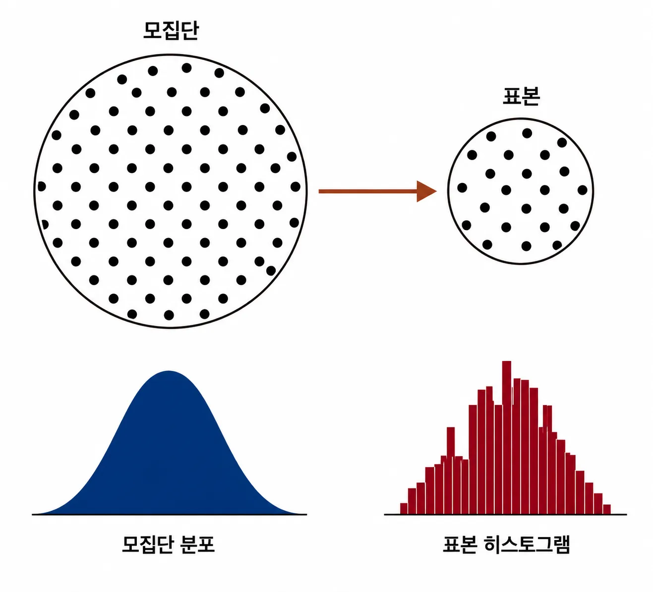
임의표본추출과 표본편향

표본: 더 **큰 데이터 집합(모집단)**으로부터 얻은 데이터의 부분집합
모집단: 어떤 데이터 집합을 구성하는 전체 대상 혹은 전체 집합
N(n): 모집단(표본)의 크기
임의표본추출(임의표집, 랜덤표본추출): 무작위로 표본을 추출하는 것
층화표본추출(층화표집): 모집단을 층으로 나눈 뒤, 각 층에서 무작위로 표본을 추출하는 것
계층: 공통된 특징을 가진 모집단의 동종 하위 그룹(복수형은 strata로 쓴다)
단순임의표본(단순랜덤표본): 모집단 층화 없이 임의표본추출로 얻은 표본
편향: 계통상의 오류
표본편향: 모집단을 잘못 대표하는 표본

통계학 모집단과 생물학 모집단의 차이가 조금 있다. 생물학에서처럼 전체 집합의 크기가 크면서도 유한한 갑승로 명확히 정의될 때도 있지만, 때로는 이론적인 가상의 집합을 의미하기도 한다.

임의표본추출: 대상이 되는 모집단 내의 선태 가능한 원소들을 무작위로 추출하는 과정을 말하며, 각 추첨에서 모든 원소는 동일한 확률로 뽑힌다. 여기서 얻은 샘플이 단순임의표본이다.
복원추출: 추출한 샘플을 다시 모집단에 포함시켜서 추출하는 기법
비복원추출: 추출한 샘플은 다시 사용하지 않는 기법

데이터 품질(완결성, 형식의 일관성, 깨끗함 및 각 데이터 값의 정확성)은 데이터의 양보다 중요하다. 통계는 여기에 대표성이라는 개념을 추가한다.

*통계에서 대표성은 추출한 표본(Sample)이나 사용하는 지표가 전체 모집단(Population)의 특성을 얼마나 정확하게 반영하는가를 뜻한다.

표본편향 사례

알프레드 랜던이 프랭클린 루스벨트를 제치고 대선에 승리하리라 예언했던 리터러리 다이제스트의 1936년 설문 조사가 아주 고전적인 사례이다. 총 1,000만 명(리터러리 다이제스트의 구독자와 그 외의 추가 명단)이 넘는 사람들을 대상으로 설문 조사를 실시하여 랜던의 승리를 예측했다. 반면, 갤럽은 겨우 2,000명을 대상으로 하는 격주 여론 조사를 실시해 루스벨트의 승리를 정확히 예측했다.

리터러리 다이제스트는 상대적으로 사회경제적 지위가 높은 사람들을 조사 대상으로 하면서 표본편향이 발생했다. 비임의 방식으로 표본추출된 것이다. 비임의는 랜덤표본이라 해도 어떤 표본도 모집단을 정확하게 대표할 수 없다는 것을 의미한다.

편향

통계적 편향은 측정 과정 혹은 표본 추출 과정에서 발생하는 계통적인 오차를 의미한다. 임의표본추출로 인한 오류와 편향에 따른 오류는 신중하게 구분해서 봐야 한다.

임의 선택

앞선 리터러리 다이제스트와 같은 사례가 나오지 않게 하려면 임의표본추출이 필요하다. 임의표본추출을 잘하기 위해서는 모집단을 적절하게 정의하는 게 매우 중요하다. 층화표본추출을 진행할 수도 있는데, 이때 특정 층의 표본이 너무 적다면, 해당 층에 높은 가중치를 주는 표본 추출을 통해 계층마다 동일한 표본크기를 얻을 수 있다.

크기와 품질: 크기는 언제 중요해질까?

빅데이터 시대라고 해도 의외로 데이터 개수가 적을수록 더 유리한 경우가 있다. 임의표본추출에 시간과 노력을 기울일수록 편향을 주링고 데이터 탐색 및 데이터 품질에 더 집중할 수 있다. 예를 들어 결측값이나 특잇값으로부터 유용한 정보를 얻을 수 있다.

그렇다면 대량의 데이터는 언제 필요한가?

데이터가 크고 동시에 희소할 때이다. 예를 들면 구글 검색의 검색 쿼리가 있다.

표본평균과 모평균

• 표본평균 기호: $\bar{x}$ (엑스 바, x-bar) • 모집단의 평균 (모평균) 기호: $\mu$ (뮤, 그리스 문자 소문자) 또는 경우에 따라 $m$

이 둘을 구분하는 이유는 표본에 대한 정보는 관찰을 통해 얻어지고, 모집단에 대한 정보는 주로 작은 표본들로부터 추론하기 때문이다.

선택편향

선택편향은 데이터를 의시적이든 무의식적이든 선택적으로 고르는 관행을 의미

선택편향: 관측 데이터를 선택하는 방식 때문에 생기는 편향
데이터 스누핑: 뭔가 흥미로운 것을 찾아 광범위하게 데이터를 살피는 것
방대한 검색 효과: 중복 데이터 모델링이나 너무 많은 예측변수를 고려하는 모델링에서 비롯되는 편향 혹은 비재현성

어떤 가설을 세우고 그것을 시험하기 위해 잘 설계된 실험을 수행한다면, 그 결과에 대해 강하게 확신할 수 있다. 이런 경우는 드물고 보통은 데이터를 가지고 데이터의 패턴을 찾고자 하는데 이때 참된 패턴인지 데이터 스누핑을 통해 나온 결과인지 알 수 없다.

선택편향의 한 형태인 방대한 검색 효과를 방지하면서 모델의 성능을 검증하기 위해서는 둘 이상의 홀드아웃 세트를 사용하면 된다. 또는 목푯값 섞기(본질적으로는 순열검정)라는 것을 추천한다.

평균으로의 회귀

평균의로의 회귀란 주어진 어떤 변수를 연속적으로 측정했을 때 나타나는 현상이다. 예외적인 경우가 관찰되면 중간 정도의 경우가 관찰되는 경향이 있다. 따라서 예외 경우를 너무 특별히 생각하고 의미를 부여하면 선택편향으로 이어질 수 있다. 평균의로의 회귀는 일종의 선택편향으로 인해 나타나는 결과이다.

통계학에서의 표본분포

통계의 포본분포라는 용어는 하나의 동일한 모집단에서 얻은 여러 샘플에 대한 표본통계량의 분포를 나타낸다. 고전 통꼐의 대부분은 (작은) 표본을 가지고 (매우 큰) 모집단을 추론하는 것과 관련 있다.

표본통계량: 더 큰 모집단에서 추출된 표본 데이터들로부터 얻은 측정 지표
데이터 분포: 어떤 데이터 집합에서의 각 개별 값의 도수분포
표본분표: 여러 표본들 혹은 재표본들로부터 얻은 표본통계량의 도수분포
중심극한정리: 표본크기가 커질수록 표본분포가 정규분포를 따르는 경향
표준오차: 여러 표본들로부터 얻은 표본통계량의 변량(개별 데이터 값들의 변량을 뜻하는 표준편차와 혼동하지 말 것)

일반적으로 표본통계량으로 어떤 것을 측정하거나 모델링하기 위해 표본을 뽑는다. 이 방법에 오류가 있을 수 있다. 그래서 우리는 표본에 따라 결과가 얼마나 달라질지(표본의 변동성)에 관심이 있다.

평균과 같은 표본통계량의 분포는 데이터 자체의 분포보다 규칙적이고 종 모양일 가능성이 높다. 통계의 기반이 되는 표본이 클수록, 그럴 가능성이 높은 것이 사실이다. 또한 표본이 클수록 표본통계량의 분포가 좁아진다.

중심극한정리

위에서 설명한 현상을 중심극한정리라고 한다. 모집단이 정규분포가 아니더라도, 표본크기가 충분하고 데이터가 정규성을 크게 이탈하지 않는 경우, 여러 표본에서 추출한 평균은 종 모양의 정규곡선을 따른다.

표준오차

표준오차는 통계에 대한 표본분포의 변동성을 한마디로 말해주는 단일 측정 지표이다. 표준오차는 표본 값들의 표준편차 $s$ 와 표본크기 $n$ 을 기반으로 한 통계량을 이용하여 추정할 수 있다.

\text{표준오차} = SE = \frac{s}{\sqrt{n}}

표본크기가 커지면 표준오차가 줄어든다. 표준오차와 표본크기 사이의 관계를 때로는 n 제곱근의 법칙이라고 한다.

실제 표준오차를 측정할 때 고려할 사항은 다음과 같다.

모집단에서 완전히 새로운 샘플들을 만히 수집.
각각의 새 샘플에 대해 통계량을 계산.
2단계에서 얻은 통계량의 표준편차 계산하여 표준오차의 추정치로 사용.

표준오차를 추정하기 위해 새 샘플을 수집하는 접근 방식은 일반적으로 불가능하다. 대신 부트스트랩 재표본을 사용할 수 있다.

부트스트랩

현재 있는 표본에서 추가적으로 표본을 복원추출하고 각 표본에 대한 통계량과 모델을 다시 계산하는 절차가 부트스트랩이다.

부트스트랩 표본: 관측 데이터 집합으로부터 얻은 복원추출 표본
재표본추출(재표집, 리샘플링): 관측 데이터로부터 반복해서 표본추출하는 과정, 부트스트랩과 순열(셔플링) 과정을 포함한다.

배깅

여러 부트스랩 샘플을 가지고 트리를 여러 개 만든 다음 각 트리에서 나온 예측값을 평균 내는(분류 문제에서는 과반수 투표를 한다) 프로세스를 배깅이라고 부른다.

재표본추출 대 부트스트래핑

재표본추출과 부트스트랩은 비슷한 의미로 사용된다. 보통 재표본추출은 여러 표본이 결합되어 비복원추출을 수행할 수 있는 순열과정을 포함한다. 부트스트랩은 항상 관측된 데이터로부터 복원추출한다는 것을 의미한다.

Data and sampling distributions

With the era of big data, many people mistakenly believe sampling is no longer necessary. Today’s situation is that data keeps growing in size while its quality and relevance cannot be guaranteed to any reliable degree. If anything, the need for sampling as a way to handle data effectively and minimize bias is growing.

The left side of the figure below represents the unknown population that statistics assumes a sample is drawn from. But all we can actually use is the sample data shown on the right and the distribution we get empirically from it. Getting from the left (population) to the right (sample) is the sampling procedure. Figure 1-1

Random sampling and sample bias

Sample: a subset of data obtained from a larger data set (the population)
Population: the entire set of subjects or the full set that makes up a data set
N(n): the size of the population (sample)
Random sampling: drawing a sample at random
Stratified sampling: dividing the population into strata and drawing randomly from each stratum
Stratum: a homogeneous subgroup of a population that shares common characteristics (plural: strata)
Simple random sample: a sample obtained by random sampling without stratifying the population
Bias: systematic error
Sample bias: a sample that misrepresents the population

A statistical population differs a little from a biological one. Sometimes, as in biology, it is clearly defined as a large but finite set, but sometimes it means a theoretical, hypothetical set.

Random sampling: the process of drawing at random from the eligible elements of the target population, where every element has the same probability of being drawn on each draw. The resulting sample is a simple random sample.
Sampling with replacement: putting each drawn observation back into the population before the next draw
Sampling without replacement: drawn observations are not used again

Data quality (completeness, consistency of format, cleanliness and accuracy of individual data values) matters more than the quantity of data. Statistics adds the concept of representativeness to this.

*In statistics, representativeness means how accurately the drawn sample, or the metric used, reflects the characteristics of the whole population.

A case of sample bias

The classic case is the Literary Digest’s 1936 poll, which predicted that Alfred Landon would beat Franklin Roosevelt in the presidential election. It surveyed more than 10 million people (Literary Digest subscribers plus additional lists) and predicted a Landon victory. Gallup, by contrast, ran a biweekly poll of only 2,000 people and correctly predicted Roosevelt’s victory.

The Literary Digest surveyed people of relatively high socioeconomic status, which created sample bias. The sample was drawn in a non-random way. Non-random here means that, even with a random sample, no sample can represent the population exactly.

Bias

Statistical bias means systematic error that arises in the measurement or sampling process. Errors due to random sampling and errors due to bias should be distinguished carefully.

Random selection

To avoid cases like the Literary Digest, random sampling is needed. Defining the population properly is crucial for doing random sampling well. You can also do stratified sampling; if one stratum has too few samples, you can oversample that stratum with higher weight to get equal sample sizes for each stratum.

Size versus quality: when does size matter?

Even in the era of big data, there are surprisingly cases where fewer data points are better. The more time and effort you put into random sampling, the more you can reduce bias and focus on data exploration and data quality. For example, you can get useful information out of missing values and outliers.

So when is a large amount of data needed?

When the data is both large and sparse. Google search queries are one example.

Sample mean versus population mean

• Symbol for the sample mean: $\bar{x}$ (x-bar) • Symbol for the population mean: $\mu$ (mu, the lowercase Greek letter) or in some cases $m$

The reason to distinguish them is that information about a sample is obtained by observation, while information about a population is mostly inferred from small samples.

Selection bias

Selection bias refers to the practice of selectively choosing data, whether consciously or unconsciously.

Selection bias: bias resulting from the way observations are selected
Data snooping: extensively hunting through data for something interesting
Vast search effect: bias or non-reproducibility resulting from repeated data modeling or modeling with too many predictor variables

If you form a hypothesis and run a well-designed experiment to test it, you can be highly confident in the result. That is rare, though; usually we look for patterns in the data we have, and then we cannot tell whether a pattern is real or a product of data snooping.

To validate a model’s performance while guarding against the vast search effect, a form of selection bias, you can use two or more holdout sets. Target shuffling (essentially a permutation test) is also recommended.

Regression to the mean

Regression to the mean is a phenomenon that appears when a given variable is measured repeatedly. An extreme observation tends to be followed by a more moderate one. So attaching too much special meaning to an extreme case can lead to selection bias. Regression to the mean is a consequence of a kind of selection bias.

Sampling distributions in statistics

The term sampling distribution of a statistic refers to the distribution of a sample statistic over many samples drawn from the same population. Much of classical statistics is concerned with making inferences about (very large) populations from (small) samples.

Sample statistic: a metric computed from sample data drawn from a larger population
Data distribution: the frequency distribution of individual values in a data set
Sampling distribution: the frequency distribution of a sample statistic over many samples or resamples
Central limit theorem: the tendency of the sampling distribution to take on a normal shape as the sample size grows
Standard error: the variability of a sample statistic over many samples (not to be confused with the standard deviation, which means the variability of individual data values)

Typically we draw a sample in order to measure or model something with a sample statistic. This approach can contain error. So we are interested in how much the result would vary from sample to sample (sampling variability).

The distribution of a sample statistic like the mean is likely to be more regular and bell-shaped than the distribution of the data itself. The larger the sample the statistic is based on, the more likely this is. Also, the larger the sample, the narrower the distribution of the sample statistic.

Central limit theorem

The phenomenon described above is called the central limit theorem. Even if the population is not normally distributed, as long as the sample size is large enough and the data does not depart too far from normality, the means drawn from many samples follow a bell-shaped normal curve.

Standard error

The standard error is a single metric that sums up the variability in the sampling distribution of a statistic. It can be estimated using a statistic based on the standard deviation $s$ of the sample values and the sample size $n$ .

\text{표준오차} = SE = \frac{s}{\sqrt{n}}

As the sample size increases, the standard error decreases. The relationship between standard error and sample size is sometimes called the square-root of n rule.

To measure the standard error in practice, you would consider the following.

Collect many brand-new samples from the population.
Compute the statistic for each new sample.
Compute the standard deviation of the statistics from step 2 and use it as the estimate of the standard error.

Collecting new samples to estimate the standard error is usually not feasible. Instead, you can use bootstrap resamples.

Bootstrap

The bootstrap is the procedure of drawing additional samples with replacement from the sample you already have, and recomputing the statistic or model for each sample.

Bootstrap sample: a sample taken with replacement from an observed data set
Resampling: the process of repeatedly drawing samples from observed data; includes both bootstrap and permutation (shuffling) procedures

Bagging

The process of building many trees from multiple bootstrap samples and then averaging the predictions from each tree (taking a majority vote for classification) is called bagging.

Resampling versus bootstrapping

Resampling and the bootstrap are used with similar meanings. Resampling usually includes permutation procedures, where multiple samples are combined and drawn without replacement. The bootstrap always means drawing with replacement from the observed data.